Diagnosing heart disease using a robust and explainable pipeline in tidyverse
One application of machine-learning in the domain of health is diagnosing a condition using descriptive information, which can lead to a particular course of treatment or the absence of treatment. In such a context health professionals and patients need to understand the process used by the model to generate a final decision or classification.
Here we use the Heart Disease UCI dataset from Kaggle including 13 features as well as a target condition of having or not having heart disease.
First, load the libraries and data
df <- read_csv("datasets_33180_43520_heart.csv")
## Parsed with column specification:
## cols(
##   age = col_double(),
##   sex = col_double(),
##   cp = col_double(),
##   trestbps = col_double(),
##   chol = col_double(),
##   fbs = col_double(),
##   restecg = col_double(),
##   thalach = col_double(),
##   exang = col_double(),
##   oldpeak = col_double(),
##   slope = col_double(),
##   ca = col_double(),
##   thal = col_double(),
##   target = col_double()
## )
Lets take a look
df = df %>%
  mutate_at(vars(sex,cp, fbs, restecg, exang, slope, ca,  thal, target), as.factor)

df
## # A tibble: 303 x 14
##      age sex   cp    trestbps  chol fbs   restecg thalach exang oldpeak slope
##    <dbl> <fct> <fct>    <dbl> <dbl> <fct> <fct>     <dbl> <fct>   <dbl> <fct>
##  1    63 1     3          145   233 1     0           150 0         2.3 0
##  2    37 1     2          130   250 0     1           187 0         3.5 0
##  3    41 0     1          130   204 0     0           172 0         1.4 2
##  4    56 1     1          120   236 0     1           178 0         0.8 2
##  5    57 0     0          120   354 0     1           163 1         0.6 2
##  6    57 1     0          140   192 0     1           148 0         0.4 1
##  7    56 0     1          140   294 0     0           153 0         1.3 1
##  8    44 1     1          120   263 0     1           173 0         0   2
##  9    52 1     2          172   199 1     1           162 0         0.5 2
## 10    57 1     2          150   168 0     1           174 0         1.6 2
## # ... with 293 more rows, and 3 more variables: ca <fct>, thal <fct>,
## #   target <fct>
Variables are as follows:
- age: The person’s age in years
- sex: The person’s sex (1 = male, 0 = female)
- cp: The chest pain experienced (Value 1: typical angina, Value 2: atypical angina, Value 3: non-anginal pain, Value 4: asymptomatic)
- trestbps: The person’s resting blood pressure (mm Hg on admission to the hospital)
- chol: The person’s cholesterol measurement in mg/dl
- fbs: The person’s fasting blood sugar (> 120 mg/dl, 1 = true; 0 = false)
- restecg: Resting electrocardiographic measurement (0 = normal, 1 = having ST-T wave abnormality, 2 = showing probable or definite left ventricular hypertrophy by Estes’ criteria)
- thalach: The person’s maximum heart rate achieved
- exang: Exercise induced angina (1 = yes; 0 = no)
- oldpeak: ST depression induced by exercise relative to rest (‘ST’ relates to positions on the ECG plot. See more here)
- slope: the slope of the peak exercise ST segment (Value 1: upsloping, Value 2: flat, Value 3: downsloping)
- ca: The number of major vessels (0-3)
- thal: A blood disorder called thalassemia (3 = normal; 6 = fixed defect; 7 = reversable defect) target: Heart disease (0 = no, 1 = yes)
As indicated here “The diagnosis of heart disease is done on a combination of clinical signs and test results. The types of tests run will be chosen on the basis of what the physician thinks is going on, ranging from electrocardiograms and cardiac computerized tomography (CT) scans, to blood tests and exercise stress tests.”
Here our pipeline includes seven steps as follows:
- Step 0
In order to implement a robust pipeline we first create training and test splits with a 10 fold cross validation structure.
df_split <- initial_split(df)
train_data <- training(df_split)
test_data <- testing(df_split)
cv_train <- vfold_cv(train_data, v = 10, repeats = 5, strata = "target")
- Step 1
Then we proceed with preprocessing using the recipe package including imputation of missing data, standardisation of numeric variables, and dummy coding of the categorical variables.
rec_obj <- recipe(target ~ ., data = df)
imputed <- rec_obj %>%
  step_knnimpute(all_predictors())
ind_vars <- imputed %>%
  step_dummy(all_predictors(), -all_numeric())
standardized <- ind_vars %>%
  step_center(all_predictors())  %>%
  step_scale(all_predictors())
- Step 2
The model development step will be implemented using the tidymodels package by setting the model, engine, and variable to be tuned in the cross-validation procedure. This starts with setting up the model:
rf_mod <-
  rand_forest(mtry = tune(), min_n = tune(), trees = 1000) %>%
  set_engine("ranger", num.threads = cores) %>%
  set_mode("classification")

rf_mod
## Random Forest Model Specification (classification)
##
## Main Arguments:
##   mtry = tune()
##   trees = 1000
##   min_n = tune()
##
## Engine-Specific Arguments:
##   num.threads = cores
##
## Computational engine: ranger
- Step 3
Development of the workflow and to implement the training step with the grid search function. Setting up the workflow:
rf_workflow <-
  workflow() %>%
  add_model(rf_mod) %>%
  add_recipe(standardized)

rf_workflow
## == Workflow ===============================================================================================================================
## Preprocessor: Recipe
## Model: rand_forest()
##
## -- Preprocessor ---------------------------------------------------------------------------------------------------------------------------
## 4 Recipe Steps
##
## * step_knnimpute()
## * step_dummy()
## * step_center()
## * step_scale()
##
## -- Model ----------------------------------------------------------------------------------------------------------------------------------
## Random Forest Model Specification (classification)
##
## Main Arguments:
##   mtry = tune()
##   trees = 1000
##   min_n = tune()
##
## Engine-Specific Arguments:
##   num.threads = cores
##
## Computational engine: ranger
and running the tune grid function
set.seed(345)
rf_res <-
  rf_workflow %>%
  tune_grid(grid = 25,
            control = control_grid(save_pred = TRUE),
            metrics = metric_set(roc_auc),
            resamples = cv_train)
- Step 4
Find the set of best performing hyperparameter using the performance metrics (collect metrics) and to select best models to fit to test data.
rf_res %>%
  collect_metrics()
rf_best <-
  rf_res %>%
  select_best(metric = "roc_auc")

rf_best

rf_res %>%
  show_best(metric = "roc_auc")

autoplot(rf_res)
- Step 5
Fit the best performing model to the test data using the last fit function.
last_rf_mod <-
  rand_forest(mtry = 1, min_n = 38, trees = 1000) %>%
  set_engine("ranger", num.threads = cores, importance = "impurity") %>%
  set_mode("classification")

last_rf_workflow <-
  rf_workflow %>%
  update_model(last_rf_mod)


set.seed(345)
last_rf_fit <-
  last_rf_workflow %>%
  last_fit(df_split)


last_rf_fit %>%
  collect_metrics()
## # A tibble: 2 x 3
##   .metric  .estimator .estimate
##   <chr>    <chr>          <dbl>
## 1 accuracy binary         0.867
## 2 roc_auc  binary         0.960
- Step 6
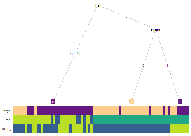
Interpretability analysis: First let’s visualize a simplified tree
heat_tree(test_data, target_lab = 'target')
## Registered S3 method overwritten by 'seriation':
##   method         from
##   reorder.hclust gclus

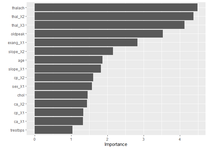
The VIP package provides model specific measure such feature importance based on class impurity for random forests
last_rf_fit %>%
  pluck(".workflow", 1) %>%
  pull_workflow_fit() %>%
  vip(num_features = 15)

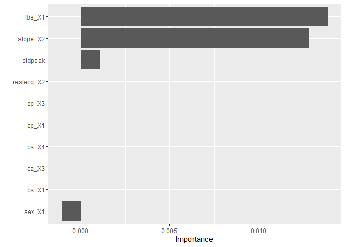
Another type of measures provided by the VIP package are model agnostic indices from permutation, ICE, or PDP, procedures. Permutation importance an index for interpreting a machine-learning model, which involves shuffling individual variables after a model has been fit and seeing the effect on accuracy.
Let’s take a look,
test_rec <- prep(standardized)%>%bake(test_data)
rfo <- ranger::ranger(target ~ ., mtry = 1, min.node.size = 38, num.trees = 1000, data = test_rec, importance = "permutation")
pfun <- function(object, newdata) predict(object, data = newdata)$predictions
vip(rfo, method = "permute", metric = "auc", pred_wrapper = pfun,
   target = "target", reference_class = 0)

