Stock Forecasting with R
Forecasting the fluctuation patterns of stock prices has been an extensively researched domain both in statistics and data science literature. Although the efficient market hypothesis asserts that it is impossible to predict stock prices, several cases established that if correctly formulated and modeled, prediction of stock prices can be done with a fairly high level of accuracy. This latter viewpoint focused on the construction of robust machine learning and statistical models based on the careful choice of variables/hyper parameters and appropriate functional forms or models of forecasting. Along the same lines a strand of research in the literature focused on time series analysis and decomposition for forecasting future values of stocks.
Previous studies attempting forecast the patterns of stock prices can be classified into three strands, according to the choice of techniques of estimation and variables used for forecasting. The first strand consists of studies using linear or non-linear regression techniques. The second strand of the previous studies following time series data and capitalizing on forecasting models and techniques to forecast stock returns like autoregressive integrated moving average (ARIMA), quantile regression (QR), autoregressive distributed lag (ARDL), and Granger causality test, to forecast stock prices. The third strand includes work using modern machine learning and deep learning tools for the prediction of stock returns.
As mentioned above, time series is referring to a series of data points ordered in time and forecasting models are optimized to predict future values based on previously observed time series based on time and other time varying or time invariant covariates independent variables. There are also other aspects that come into play when dealing with time series. Is the time series stationary? Is the dependant variable autocorrelated? Is there a seasonality in the time series?
Stationarity
A time series is said to be stationary if its statistical properties do not change over time. Stationarity is essential as in its absence, the model forcasting the data will vary in performance at different time points. Therefore, stationarity is required for sample statistics such as means, variances, and correlations to accurately describe the data at all time points of interest.
Autocorrelation
Autocorrelation measures the relationship between a variable’s current value and its past values. In other words, it is the relationship between observations based on the time lag between them that can be represented in a plot looks like sinusoidal function. This means that we will find a very similar value at a given lagged unit of time (e.g., once in each 12th observation).
Seasonality
Seasonality refers to periodic fluctuations in time series data that is characterized by the presence of variations that occur at specific regular intervals. For example, natural consumption is high during the winter and low during summer, or online sales increase during black Friday weekend before slowing down again. Seasonality can be derived from an autocorrelation plot with a sinusoidal shape. Simply look at the period, and it gives the length of the season.
An important note is that stock return is not always stationary. As mentioned above, non-stationary processes have variable mean and variance, in contrast to stationary processes that reverts around a constant long-term mean and has a constant variance independent of time. Generally, non-stationary data, cannot be forecasted or modeled with traditional forecasting methods. Modelling non-stationary time series data may result in spurious associations in that they may indicate a relationship where one does not exist. Along these lines, to receive consistent, reliable results, the non-stationary data needs to be transformed into stationary data. Similarly autocorrelation and seasonality of stocks data have been discussed thoroughly in the literature.
Here we are going to focus on forecasting of an equity return using the tidy model framework and focusing on longitudinal cross-validation, which can be implemented with parameter tuning. The analyzed index used here will be BTC, the conversion rate of bitcoin to USD, with data extracted from Yahoo Finance using the package quantmod in R.
library(PerformanceAnalytics)
library(quantmod)
library(tidyverse)
library(modeldata)
library(forecast)
library(tidymodels)
library(modeltime)
library(timetk)
library(lubridate)
BTC <- getSymbols("BTC-USD", src = "yahoo", from = "2013-01-01", to = "2020-11-01", auto.assign = FALSE)
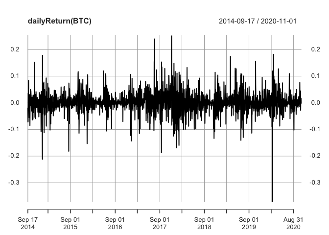
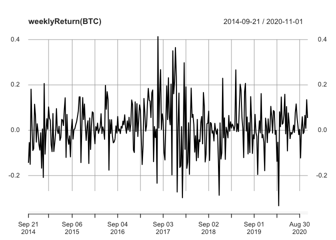
A possibility given by quantmod is the calculation of returns for different periods. For example, it’s possible to calculate the returns by day, week, month, quarter and year, just by using the following commands:
plot(dailyReturn(BTC))
plot(weeklyReturn(BTC))
 Here we add the date column to the time-series data set.
ts=as.data.frame(dailyReturn(BTC))
ts$date=as.Date (row.names(ts))
and split the data to trining and test fro cross validation.
train_data <- training(initial_time_split(ts, prop = .8))
test_data <- testing(initial_time_split(ts, prop = .8))
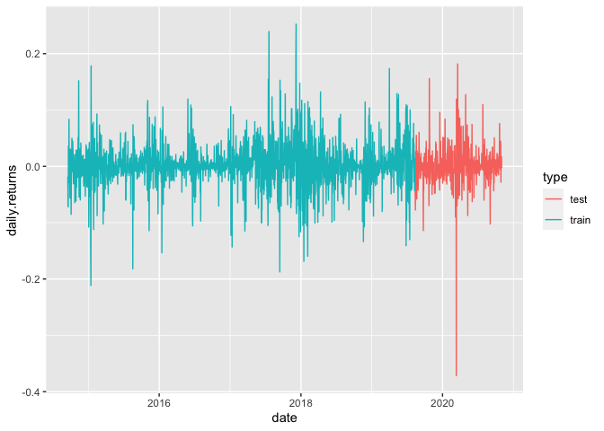
Here is the visualization of propre training test split for time series data.
train_data %>% mutate(type = "train") %>%
  bind_rows(test_data %>% mutate(type = "test")) %>%
  ggplot(aes(x = date, y =daily.returns, color = type)) +
  geom_line()
The model fitting procedure is similar to that tidy models, here is the example for an ARIMA model fitted on the training data,
arima_model <- arima_reg() %>%
  set_engine("auto_arima") %>%
  fit(daily.returns~date, data = train_data)
## frequency = 7 observations per 1 week
a prophet regression model fitted on the training data,
prophet_model <- prophet_reg() %>%
  set_engine("prophet") %>%
  fit(daily.returns~date, data = train_data)
## Disabling daily seasonality. Run prophet with daily.seasonality=TRUE to override this.
and a linear regression model fitted on the training data.
tslm_model <- linear_reg() %>%
  set_engine("lm") %>%
  fit(daily.returns~as.numeric(date) + factor(month(date, label = TRUE)), data = train_data)
In order to put all the results together and compare them you have to creat a tibble of the model out comes.
forecast_table <- modeltime_table(
  arima_model,
  prophet_model,
  tslm_model
)
Then to compare the performances the models should be fitted on the test data.
forecast_table %>%
  modeltime_calibrate(test_data) %>%
  modeltime_accuracy()
## # A tibble: 3 x 9
##   .model_id .model_desc            .type    mae  mape  mase smape   rmse     rsq
##       <int> <chr>                  <chr>  <dbl> <dbl> <dbl> <dbl>  <dbl>   <dbl>
## 1         1 ARIMA(0,0,0)(1,0,1)[7… Test  0.0214  150. 0.640  162. 0.0356 2.17e-4
## 2         2 PROPHET                Test  0.0217  182. 0.648  158. 0.0356 4.84e-3
## 3         3 LM                     Test  0.0218  205. 0.651  153. 0.0358 1.00e-3
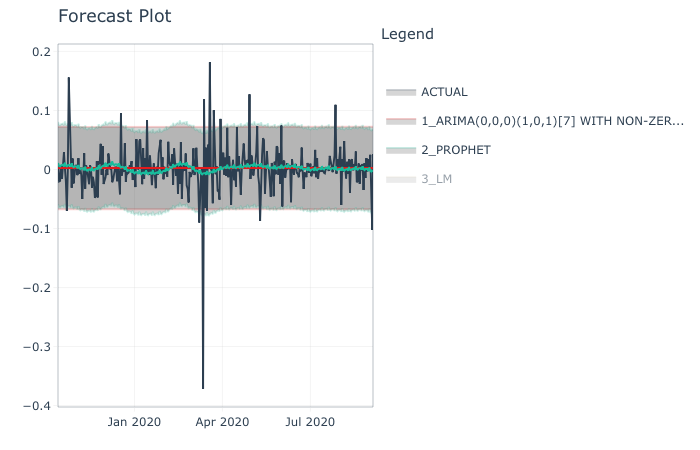
it is also possible to plot the comparative performance .
forecast_table %>%
  modeltime_calibrate(test_data) %>%
  modeltime_forecast(actual_data = test_data) #%>%
  plot_modeltime_forecast()
