Update 1: The Landscape of R packages for eXplainable Artificial Intelligence can be found here
Feature Importance Analysis in R
In new the era of machine learning and data science, there is an emerging challenge to build state-of-the-art predictive models that also provide an understanding of what’s really going on under the hood and in the data. Therefore, it is often of interest to know which, of the predictors in a fitted model are relatively influential on the predicted outcome. There are many methodologies to interpret machine learning results (i.e., variable importance via permutation, partial dependence plots, local interpretable model-agnostic explanations), and many machine learning R packages implement their own versions of one or more methodologies. However, some recent R packages that focus purely on ML interpretability agnostic to any specific ML algorithm are gaining popularity. As a part of a larger framework referred to as interpretable machine learning (IML), VIP is an R package for constructing variable importance plots (VIPs).
here for our example we use the diabetes data from pdp package
data(pima, package = "pdp")
out="diabetes"
preds=colnames(pima)[-c(9)]
df=pima%>%
  select(c(out,preds))%>%
  drop_na()
table(df$diabetes)
##
## neg pos
## 262 130
first data is divided to train and test sets and pre-processing is done with the Recipes package
df_split <- initial_split(df)
train_data <- training(df_split)
test_data <- testing(df_split)
cv_train <- vfold_cv(train_data, v = 5, repeats = 2, strata = out)

standardized <- recipe(diabetes ~ ., data = train_data)%>%
  step_center(all_predictors())  %>%
  step_scale(all_predictors()) %>%
  themis::step_smote (diabetes)
train_preped <- prep(standardized) %>%
  bake(new_data = NULL)

test_preped <-  prep(standardized) %>%
  bake(new_data = test_data)


require(doParallel)

cores <- parallel::detectCores(logical = FALSE)
registerDoParallel(cores = cores)
then we fine tune a random forest model using the tidymodels framework
rf_mod <-
  rand_forest(mtry = tune(), min_n = tune(), trees = tune()) %>%
  set_engine("ranger", num.threads = cores) %>%
  set_mode("classification")

rf_mod
## Random Forest Model Specification (classification)
##
## Main Arguments:
##   mtry = tune()
##   trees = tune()
##   min_n = tune()
##
## Engine-Specific Arguments:
##   num.threads = cores
##
## Computational engine: ranger
rf_workflow <-
  workflow() %>%
  add_model(rf_mod) %>%
  add_recipe(standardized)

rf_workflow
## ══ Workflow ════════════════════════════════════════════════════════════════════
## Preprocessor: Recipe
## Model: rand_forest()
##
## ── Preprocessor ────────────────────────────────────────────────────────────────
## 3 Recipe Steps
##
## • step_center()
## • step_scale()
## • step_smote()
##
## ── Model ───────────────────────────────────────────────────────────────────────
## Random Forest Model Specification (classification)
##
## Main Arguments:
##   mtry = tune()
##   trees = tune()
##   min_n = tune()
##
## Engine-Specific Arguments:
##   num.threads = cores
##
## Computational engine: ranger
set.seed(345)
rf_res <-
  rf_workflow %>%
  tune_grid(grid = 10,
            control = control_stack_grid(),
            metrics = metric_set(roc_auc,f_meas,sens,bal_accuracy),
            resamples = cv_train)
rf_res %>%
  collect_metrics()
rf_best <-
  rf_res %>%
  select_best(metric = "f_meas")

rf_best
rf_res %>%
  show_best(metric = "f_meas")
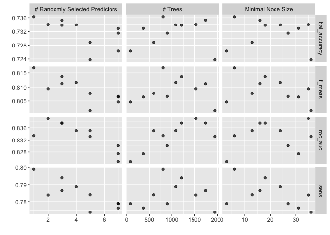
autoplot(rf_res)
final_rf <- finalize_model(
  rf_mod,
  rf_best
)

final_rf
## Random Forest Model Specification (classification)
##
## Main Arguments:
##   mtry = 1
##   trees = 798
##   min_n = 6
##
## Engine-Specific Arguments:
##   num.threads = cores
##
## Computational engine: ranger
Global Measures
Model-Based Variable Importance
Many supervised learning algorithms can naturally emit some measure of importance for the features used in the model, and these approaches are embedded in many different packages. For instance, like gradient boosted decision trees and random forests have a native way of quantifying the importance or relative influence of each feature. These measures compute variable importance specific to the particular model from the native functions of a wide range of packages.
final_rf %>%
  set_engine("ranger", importance = "impurity") %>%
  fit(diabetes ~ .,
      data = train_preped
  ) %>%
  vi()%>%mutate(rank = dense_rank(desc(Importance)),
                mod="rf")%>% select(Variable,rank,mod)
Permutation Method
The permutation method exists in various forms the approach used in the VIP package is quite simple. The idea is as permuting the values of a feature affects the relationship between that feature and the target variable if we randomly permute the values of an important feature in the training data, the training performance would decrease. This approach uses the difference between the performance of the baseline full model and the performance obtained after permuting the values of a particular feature.
pfun <- function(object, newdata) predict(object, data = newdata)$predictions
vips=final_rf %>%
 set_engine("ranger", importance = "impurity") %>%
 fit(diabetes ~ .,
     data = train_preped
 ) %>%
 vi(method = "permute", nsim = 100, target = "diabetes",
    pred_wrapper = pfun, metric = "accuracy",
    all_permutations = TRUE, train = train_preped)
FIRM
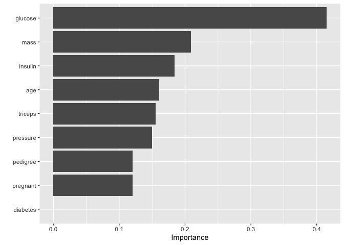
FIRM-based variable importance - Compute variable importance by quantifying the variability in marginal effect plots like Partial Dependence Plots and Individual Conditional Expectations via the pdp package.
final_rf %>%
  set_engine("ranger", importance = "permutation") %>%
  fit(diabetes ~ .,
      data = train_preped
  ) %>%vip( method = "firm",feature_names = setdiff(names(train_preped), "outcome"), train = train_preped)
PDP Method
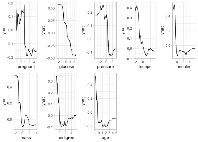
Partial Dependence Plots provide model-agnostic interpretations and can be constructed in the same way for any supervised learning algorithm. This approach is based on quantifying the “flatness” of the PDPs of each feature by visualizing the effect of cardinality of the subsets of the feature space on the estimated.
pdp_DBT<- model_profile(
  rf_explainer,
  variables = "mass",
  N = NULL
)
# pdp_DBT
#
#
# as_tibble(pdp_DBT$agr_profiles) %>%
#   mutate(`_label_` = str_remove(`_label_`, "workflow_")) %>%
#   ggplot(aes(`_x_`, `_yhat_`, color = `_label_`)) +
#   geom_line(size = 1.2, alpha = 0.8)

pp=final_rf %>%
  set_engine("ranger", importance = "permutation") %>%
  fit(diabetes ~ .,
      data = train_preped
  )

features <- setdiff(names(train_preped), "diabetes")
pdps <- lapply(features, FUN = function(feature) {
  pd <- partial(pp$fit, pred.var = feature,train=train_preped)
  autoplot(pd) +
    theme_light()
})
grid.arrange(grobs = pdps, ncol = 5)
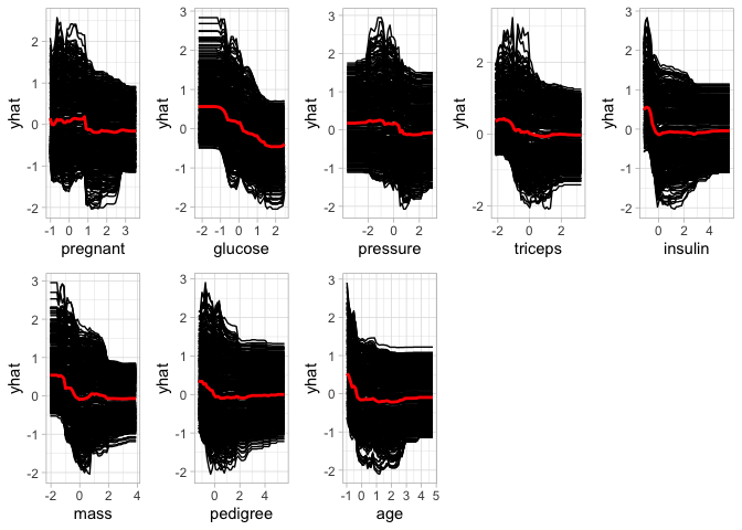
ICE curve Method
The Individual Conditional Expectations curve method is similar to the PDP method, however, in this approach the “flatness” of each ICE curve and then aggregate the results (e.g., by averaging). Therefore, in absence of interaction effects, using method = “ice” will produce results similar to using method = “pdp”. Some would argue that it is probably more reasonable to always use method = “ice”.
features <- setdiff(names(train_preped), "diabetes")
ices <- lapply(features, FUN = function(feature) {
  ice <- partial(pp$fit, pred.var = feature,train=train_preped, ice = TRUE)
  autoplot(ice) +
    theme_light()
})

grid.arrange(grobs = ices, ncol = 5)
Local Measures
Global interpretations are based on the relationship between the features and the outcome in the entire model. However, global measures can be highly approximate in some cases. Local measures, in contrast, highlight model predictions for a single observation or a group of similar observations. Local interpretability measures like SHAP-based variable importance and LIME, which stands for Local Interpretable Model-agnostic Explanations, has the potential to facilitate the interpretation of black-box models.
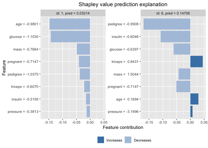
SHAP
Similar to LIME method, Lundberg et al. in their paper “A unified approach to interpreting model predictions” proposed the SHAP (SHapley Additive exPlanations). The SHAP values can provide global interpretability about how much each predictor contributes, either positively or negatively, to the target variable, as well as local interpretability measures where each observation gets its own set of SHAP values which increases its transparency of the model. In contrast to LIME method that creates a substitute model around the local unit to understand. Shapely values ‘decompose’ the final prediction into the contribution of each attribute in an additive way.
x_train <- as.matrix(train_preped[-1:-6, 1:8])
y_train <- as.matrix(train_preped[-1:-6, 9])
x_test <- as.matrix(train_preped[1:6, 1:8])
explainer <- shapr(x_train, pp$fit)
## The specified model provides feature classes that are NA. The classes of data are taken as the truth.
p <- mean(as.numeric(as.factor(y_train))-1)
explanation <- explain(
  x_test,
  approach = "empirical",
  explainer = explainer,
  prediction_zero = p
)

plot(explanation, plot_phi0 = FALSE, index_x_test = c(1, 6))
LIME
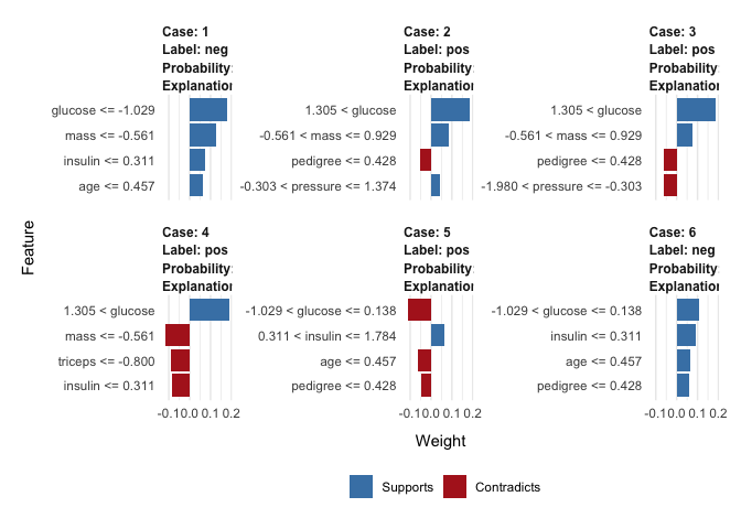
Local Interpretable Model-agnostic Explanations (LIME) is a model agnostic method that can be applied to any supervised regression or classification model, based on the the assumption that every complex model is linear on a local scale. In other words, it is possible to fit a simple model around a single observation that will mimic how the global model behaves at that locality. To attain this lime permute features for a given observation and computes similarity distance measure between original observation and permuted observations and then applies selected machine learning model to predict outcomes of permuted data.
explainer <- lime(as.data.frame(x_train), pp$fit, bin_continuous = TRUE, quantile_bins = FALSE)
explanation <- lime::explain(as.data.frame(x_test), explainer, n_labels = 1, n_features = 4)
plot_features(explanation, ncol = 3)
