Twitter Analysis with R

Twitter APIs are one of the easily available and retrievable sources of user-generated language data that provides the opportunity to gain insights into the online public behaviour of a given person or around a given subject of matter. Hence, getting access and analysing Twitter has become a crucial source of information for both scientific and business investigations. Twitter has considerable advantages over other social media platforms for analysis of the text data because of the large number of tweets published every day that allows access to large data samples as well as the size of the tweets leading to a relatively homogeneous corpus. However, extracting the insights still requires coding, this article provides a simple guide on how to extract and analyse tweets with the R programming software.

Step 1:

Load the required packages (including rtweet) in RStudio

library(rtweet)        
library(tm)            
library(stringr)       
library(qdapRegex)     
library(wordcloud2)    
library(tidytext)
library(dplyr)
library(stopwords)
library(PersianStemmer)
library(tidyr)
library(stringr)
library(igraph)
library(ggraph)
library(textdata)

Step 2:

Authenticate using your credentials to Twitter’s API by creating an access token. In order to get started, you first need to get a Twitter API that allows you to retrieve the tweets. To get a Twitter API you have to use your Twitter account and apply for a developer account via the website here. There is an application form to be accepted by Twitter. Once accepted, you’ll receive the following credentials that you need to keep safe:

Consumer key:#######################
Consumer Secret:#######################
Access Token:#######################
Access Secret:#######################

token=create_token(
  app = "#######################",
  consumer_key = "#######################",
  consumer_secret = "#######################",
  access_token = "##############################################",
  access_secret = "#######################")
token

## <Token>
## <oauth_endpoint>
##  request:   https://api.twitter.com/oauth/request_token
##  authorize: https://api.twitter.com/oauth/authenticate
##  access:    https://api.twitter.com/oauth/access_token
## <oauth_app> #######################
##   key:    #######################
##   secret: <hidden>
## <credentials> oauth_token, oauth_token_secret
## ---

head(rtweet::trends_available())

name	url	parentid	country	woeid	countryCode	code	place_type
Worldwide	http://where.yahooapis.com/v1/place/1	0		1	NA	19	Supername
Winnipeg	http://where.yahooapis.com/v1/place/2972	23424775	Canada	2972	CA	7	Town
Ottawa	http://where.yahooapis.com/v1/place/3369	23424775	Canada	3369	CA	7	Town
Quebec	http://where.yahooapis.com/v1/place/3444	23424775	Canada	3444	CA	7	Town
Montreal	http://where.yahooapis.com/v1/place/3534	23424775	Canada	3534	CA	7	Town
Toronto	http://where.yahooapis.com/v1/place/4118	23424775	Canada	4118	CA	7	Town

## Step 3:

Search tweets on the topic or person of your choice to limit the number of tweets as you see fit and decide on whether or not to include retweets. You can do the same analysis with the hashtags. In this case, you’ll want to use the hashtags variable from the rtweet package. Here we included 5000 tweets the ChristophMolnar twitter account.

tweets_CM <- get_timelines(c("ChristophMolnar"), n = 5000)
text <- str_c(tweets_CM$text, collapse = "")

Step 4:

The next step is to pre-process set of tweets into tidy text or corpus objects or simply put to clean up the tweets this includes converting all words to lower-case, removing links to web pages (http elements), hashtags, and mnetions using @ sign, as well as deleting punctuation and stop words. Here we use the tidytext and stopwords packages to remove the words from the tweets that are not helpful in the overall analysis of a text body such as “I”, “ myself”, “ themselves”, “being” and “have”.

text <- 
  text %>%
  str_remove("\\n") %>%                  
  rm_twitter_url() %>%                   
  rm_url() %>%
  str_remove_all("#\\S+") %>%             
  str_remove_all("@\\S+") %>%             
  removeWords(c(stopwords("english"))) %>%  
  removeNumbers() %>%
  stripWhitespace() %>%
  removeWords(c("amp", "the"))          


textCorpus <- 
  Corpus(VectorSource(text)) %>%
  TermDocumentMatrix() %>%
  as.matrix()

Step 5:

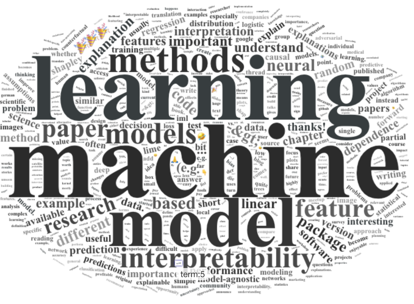
The word frequency table can be visualized using a word cloud as shown below.

textCorpus <- sort(rowSums(textCorpus), decreasing=TRUE)
textCorpus <- data.frame(word = names(textCorpus), freq=textCorpus, row.names = NULL)
textCorpus=textCorpus[textCorpus$freq>4,]
textCorpus=textCorpus[-c(which(as.vector(textCorpus$word)%in%stopwordslangs$word[stopwordslangs$lang=="en"][1:500])),]

yellowPalette <- c("#2B2B2B", "#373D3F", "#333333", "#303030", "#404040", "#484848", "#505050", "#606060", 
                   "#444444", "#555555", "#666666", "#777777", "#888888", "#999999")

wordcloud <-wordcloud2(data = textCorpus, color=rep_len( yellowPalette, nrow(textCorpus)))
#wordcloud

Step 6:

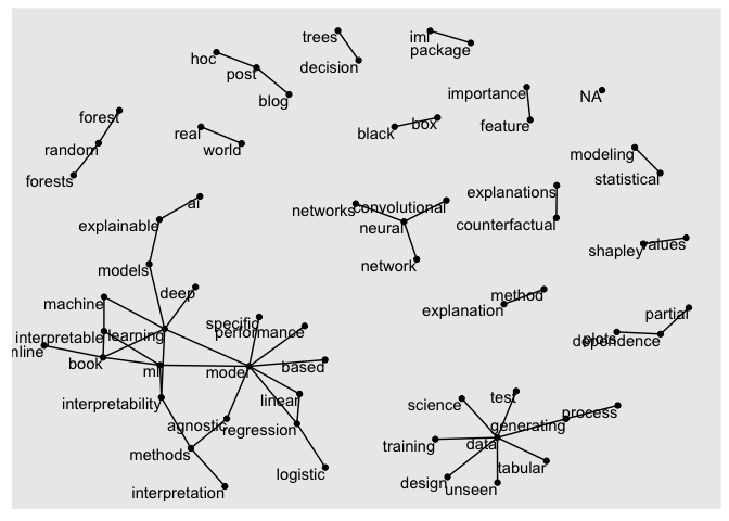
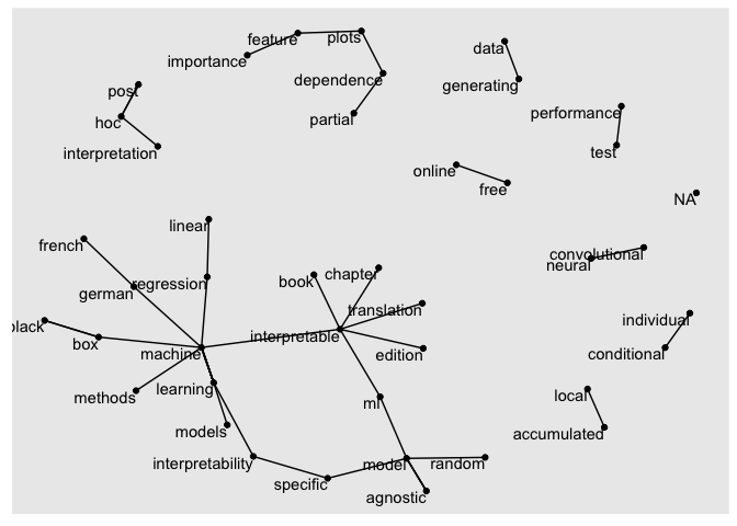
Bigram analysis: Rather than looking at individual words it is also possible to examine cooccurance between terms. Based on the cleaned data we have to transform from long to wide and extract the bigrams.

tweets_CM2=as.data.frame(tweets_CM[,c(1,5)])

tweets_CM2$text <- 
  tweets_CM2$text %>%
  str_remove("\\n") %>%                  
  rm_twitter_url() %>%                   
  rm_url() %>%
  str_remove_all("#\\S+") %>%             
  str_remove_all("@\\S+") %>%             
  removeWords(c(stopwords("english"))) %>%  
  removeNumbers() %>%
  stripWhitespace() %>%
  removeWords(c("amp", "the"))          

d <- tibble(txt = tweets_CM2$text)
CM_bigrams <- d %>% unnest_tokens(bigram, txt, token = "ngrams", n = 2)


bigrams_separated <- CM_bigrams %>%
  separate(bigram, c("word1", "word2"), sep = " ")
bigrams_filtered <- bigrams_separated %>%
  filter(!word1 %in% stop_words$word) %>%
  filter(!word2 %in% stop_words$word)

bigram_counts <- bigrams_filtered %>% 
  count(word1, word2, sort = TRUE)

#bigram_counts


bigram_graph <- bigram_counts %>%
  filter(n > 5) %>%
  graph_from_data_frame()

set.seed(2017)
ggraph(bigram_graph, layout = "fr") +
  geom_edge_link() +
  geom_node_point() +
  geom_node_text(aes(label = name), vjust = 1, hjust = 1)

trigrams <- d %>% unnest_tokens(trigram, txt, token = "ngrams", n = 3)
trigram_counts=
  trigrams %>%
  separate(trigram, c("word1", "word2", "word3"), sep = " ") %>%
  filter(!word1 %in% stop_words$word,
         !word2 %in% stop_words$word,
         !word3 %in% stop_words$word) %>%
  count(word1, word2, word3, sort = TRUE)
trigram_graph <- trigram_counts %>%
  filter(n >2) %>%
  graph_from_data_frame()

set.seed(2017)

ggraph(trigram_graph, layout = "fr") +
  geom_edge_link() +
  geom_node_point() +
  geom_node_text(aes(label = name), vjust = 1, hjust = 1)

#trigram_graph
#bigram_graph

Step 7:

There are many libraries, dictionaries and packages available in R to perform sentiment analysis which is to evaluate the emotion prevalent in a text. Here we use textdata and tidytext packages for word-to-emotion evaluation using two dictionaries namely Bing, AFINN. The get_sentiments function returns a tibble with either “positive” and “negative” sentiment or a numerical value, where a calculated score of zero indicates neutral sentiment, a score greater than zero indicates positive sentiment, while a score less than zero would mean negative overall emotion.

mat=as.data.frame(as.matrix(TermDocumentMatrix(Corpus(VectorSource(tweets_CM2$text)))))
mat$word=row.names(mat)
mat=data.table::as.data.table(mat)
mat2=data.table::melt(mat,id.vars="word")
mat3= mat2 %>% inner_join(get_sentiments("afinn"))

## Joining, by = c("word", "value")

mat4= mat2 %>% 
  inner_join(get_sentiments("nrc") %>% 
               filter(sentiment %in% c("positive", 
                                       "negative"))) 

## Joining, by = "word"

mat5= mat2 %>% 
  inner_join(get_sentiments("bing"))

## Joining, by = "word"

pp=aggregate(value~word, data=mat4[mat4$sentiment=="positive",],sum)
head(pp[rev(order(pp$value)),])%>%kableExtra::kable()

	word	value
239	learning	211
258	model	164
174	good	94
142	feature	59
197	important	32
219	interesting	26

##nn=aggregate(value~word, data=mat4[mat4$sentiment=="negative",],sum)
##head(nn[rev(order(nn$value)),])

kamran Afzali's Portfolio

Twitter Analysis with R