Introduction
Any organisation must be able to recognise time-based patterns. Questions such as how much resources to keep on hand and how much traffic to expect are crucial time series problems to address. This is why time series forecasting is incorporated into the data science ecosystem, from weather prediction to product sales, making it a technique that every data scientist should be familiar with. It. If you’re a beginner, time series is a great method to get started on real-world tasks. Time series are very easy to understand and relate to, and they assist you in entering the bigger world. Prophet is a Facebook-developed open source library based on decomposable (trend+seasonality+holidays) models. It allows us to construct accurate time series projections using simple understandable parameters, and it even allows us to factor in the influence of custom seasonality and holidays! In this post, we’ll go over some background on Prophet and how it fills in the gaps in making fast, credible forecasts, followed by a R example.
What is Prophet?
When a forecasting model fails to perform as expected, we want to be able to fine-tune the method’s parameters to fit the unique scenario at hand. Tuning these strategies necessitates a detailed understanding of the time series models that underpin them. The maximum orders of the differencing, the auto-regressive components, and the moving average components, for example, are the first input parameters to automated ARIMA. A typical analyst would have no idea how to change these instructions to avoid the behaviour, and this is the kind of knowledge that is difficult to acquire and scale.
The Prophet programme has intuitive parameters that are simple to tweak in order to create relevant predictions for a variety of business challenges. Here you’ll learn the fundamentals of using Facebook’s sophisticated forecasting tool to develop your first model and then dive further into it. Prophet is a process for forecasting time series data using an additive model, with support for trends, seasonality, and holidays. It works best with time series with substantial seasonal influences and historical data from multiple seasons. Prophet is forgiving of missing data and trend shifts, and it usually handles outliers well.
Facebook Prophet is an open-source toolkit containing R and Python APIs developed by Facebook’s Core Data Science team. It appeals to novice users because of its ease of use and ability to identify an appropriate set of hyperparameters for the model automatically. As a result, even individuals with no prior knowledge or expertise forecasting time series data may use it and receive pretty decent results that are often on par with, if not better than, those provided by professionals.
The Prophet Forecasting Model
Prophet employs a three-part decomposable time series model: trend, seasonality, and holidays.
-
g(t): non-periodic changes in time series are modelled using a piecewise linear or logistic growth curve.
-
s(t): regular changes (weekly/yearly seasonality, for example).
-
h(t): the effects of holidays (given by the user) on irregular schedules.
-
(t): error term accounts for any unexpected changes that the model does not account for.
Prophet is trying to fit numerous linear and non linear time functions as components using time as a regressor. Seasonality is modelled as an additive component in the same way that exponential smoothing is used in the Holt-Winters technique. Instead of directly looking at the time based dependence of each observation inside a time series, we are effectively framing the forecasting problem as a curve-fitting exercise.
Trend
A piecewise linear curve is fitted over the trend or non-periodic section of the time series to model the trend. The linear fitting procedure ensures that spikes and missing data are minimised.
Saturating growth
Is it reasonable to expect the target to continue growing/falling throughout the duration of the prediction interval? There are frequently situations of non-linear development with a running maximum capacity. An analyst can then define a variable capacity C(t) for the time series forecasts he or she is seeking to create using domain knowledge.
Changepoints
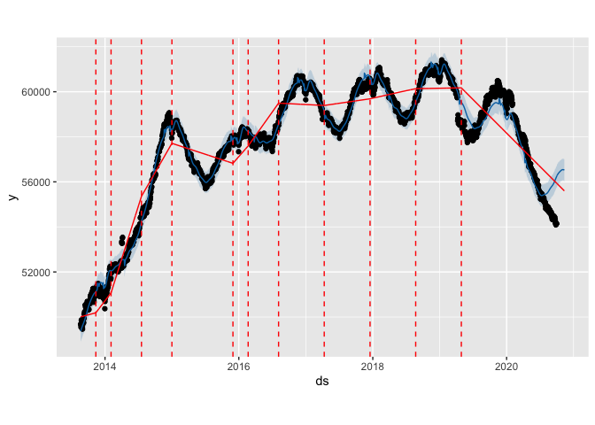
Another point to address is whether my time series encounters any underlying changes in the phenomena, such as a new product launch, a natural disaster, or other unforeseen events. The growth rate is allowed to fluctuate at such times. These changepoints are chosen at random. However, if necessary, a user can manually feed the changepoints. The dotted lines in the plot below reflect the changepoints for the provided time series. The fit becomes more adjustable as the number of changepoints allowed increases. When working with the trend component, an analyst may encounter one of two issues.
Seasonality
Prophet uses fourier series to fit and forecast the impacts of seasonality and give a flexible model. The following function approximates seasonal impacts s(t):
The letter P stands for period (365.25 for yearly data and 7 for weekly data)
An important parameter to choose here is the fourier order N, which determines whether high frequency variations can be represented. If the user considers the high frequency components in a time series are just noise and should not be included for modelling, he or she can reduce the amount of N. If not, N can be raised to a greater amount and the forecast accuracy used to set it.
Holidays and events
Holidays and events cause predictable peaks and valleys in a time series. Diwali, for example, is celebrated on a different day each year in India, and a huge section of the population buys a lot of new products during this time.
The analyst can create a custom list of past and future occurrences using Prophet. Additional parameters are fitted to model the effect of vacations and events in a window surrounding such days.
Data
Here we use daily shelter demande data, dates should be formated and time series specified.
Prophet requires a dataframe with two columns as input:
- datetime column (ds)
- y: The forecasted measurement is represented by a number column. Our data is nearly complete. All we have to do now is rename the columns date and sales to ds and y, respectively.
data <- read.csv("https://raw.githubusercontent.com/Kamran-Afzali/Statistical-Supplementary-Materials/master/DHS_Daily_Report.csv")

data$Date = strptime(data$Date, "%m/%d/%Y")
data$Date = as.Date(data$Date)
library(dplyr)
data = data %>% select("Date",
                       "Total.Individuals.in.Shelter",
                       "Easter",
                       "Thanksgiving",
                       "Christmas")
colnames(data)[2] = "y"
dataset <- subset(data, data$Date <= '2020-11-11')
library(lubridate)
dataset$y <- ts(dataset$y,
                frequency = 365,
                start =c(2013, yday(head(dataset$Date, 1))))
head(dataset)%>%kableExtra::kable()
| Date | y | Easter | Thanksgiving | Christmas |
|---|---|---|---|---|
| 2013-08-21 | 49673 | 0 | 0 | 0 |
| 2013-08-22 | 49690 | 0 | 0 | 0 |
| 2013-08-23 | 49548 | 0 | 0 | 0 |
| 2013-08-24 | 49617 | 0 | 0 | 0 |
| 2013-08-25 | 49858 | 0 | 0 | 0 |
| 2013-08-26 | 49877 | 0 | 0 | 0 |
then we split training and test sets,
training_set = subset(dataset, dataset$Date <= '2020-09-30')
test_set = subset(dataset, dataset$Date > '2020-09-30')
training_set$y <- ts(training_set$y,
                     frequency = 365,
                     start = c(2013, yday(head(training_set$Date, 1))))
test_set$y <- ts(test_set$y,
                 frequency = 365,
                 start = c(2020, yday(head(test_set$Date, 1))))
and creat the dynamic table for holidays.
library(dplyr)
easter_dates = subset(data, data$Easter == 1)
easter_dates = easter_dates$Date
easter <- tibble(holiday = 'Easter',
                 ds = as.Date(easter_dates),
                 lower_window = -3, upper_window = 1)

#Thanksgiving
thanksgiving_dates = subset(data, data$Thanksgiving == 1)
thanksgiving_dates = thanksgiving_dates$Date
thanksgiving <- tibble(holiday = 'Thanksgiving',
                 ds = as.Date(thanksgiving_dates),
                 lower_window = -7, upper_window = 4)

#Christmas
christmas_dates = subset(data, data$Christmas == 1)
christmas_dates = christmas_dates$Date
christmas <- tibble(holiday = 'Xmas',
                 ds = as.Date(christmas_dates),
                 lower_window = -4, upper_window = 3)

#Merging all holidays
holidays <- bind_rows(easter, thanksgiving, christmas)

head(holidays)%>%kableExtra::kable()
| holiday | ds | lower_window | upper_window |
|---|---|---|---|
| Easter | 2014-04-20 | -3 | 1 |
| Easter | 2015-04-05 | -3 | 1 |
| Easter | 2016-03-27 | -3 | 1 |
| Easter | 2017-04-16 | -3 | 1 |
| Easter | 2018-04-01 | -3 | 1 |
| Easter | 2019-04-21 | -3 | 1 |
Fit
In Prophet, we build an instance of the model class and then call the fit method to train a model.
You don’t need to specify any hyparameters in theory. Seasonality mode is an important exception. Because Prophet is based on an additive model, it’s critical to adjust this value to multiplicative if your model is multiplicative. Seasonality in our model follows an additive pattern, as we previously witnessed. As a result, setting seasonality mode to multiplicative is unnecessary. Although Prophet can select a suitable set of hyperparameters automatically, we shall see later how careful adjustment can increase performance. Even while Prophet has the ability to handle many things on its own, using your expertise of the business case could make a big difference.
library(prophet)
## Loading required package: Rcpp
## Loading required package: rlang
m <- prophet(growth = "linear",
             holidays = holidays,
             yearly.seasonality = TRUE,
             weekly.seasonality = FALSE,
             daily.seasonality = FALSE,
             seasonality.prior.scale = 0.001,
             changepoint.prior.scale = 0.01,
             holidays.prior.scale = 1)
here we fit the model.
df = training_set %>% select(Date, y)
colnames(df)[1] <- "ds"
m = fit.prophet(m, df)
Forecast Dataframe
To forecast, we must first establish a dataframe in which we will record our forecasts. The method make future dataframe creates a dataframe that extends a specified number of days into the future. We can observe that the model fits because the dataframe provided by default includes the dates from the history.
To make predictions, we use the procedure predict on the newly created future dataframe.
test_period <- make_future_dataframe(m, periods = nrow(test_set))
tail(test_period)%>%kableExtra::kable()
| ds | |
|---|---|
| 2635 | 2020-11-06 |
| 2636 | 2020-11-07 |
| 2637 | 2020-11-08 |
| 2638 | 2020-11-09 |
| 2639 | 2020-11-10 |
| 2640 | 2020-11-11 |
Prophet’s predications are contained in the forecast dataframe. Forecast dataframe includes a column for the forecast, as well as columns for components and uncertainty intervals.
prophet_forecast <- predict(m, test_period)
Forecast Plot
You only need to call method to plot the forecast. On your predicted dataframe, use plot().
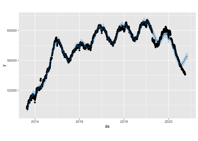
The deep blue line in the forecast plot above represents the forecast sales forecast [‘y hat’], while the black dots represent the actual sales forecast[‘y’]. Around the forecast, the light blue hue represents the 95 percent confidence interval. Forecast [‘yhat lower’] and forecast [‘yhat upper’] values define the uncertainty interval in this location.
plot(m, prophet_forecast)

Seasonality
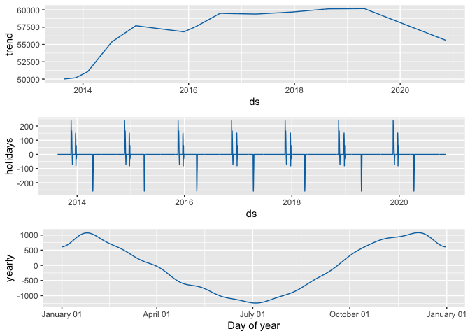
The weekly seasonality component demonstrates patterns related to weekdays, and yearly seasonality demonstrates patterns related to different times of the year. To improve your model, look at holidays, special events, and seasonality. Check to Prophet’s documentation section Seasonality, Holiday Effects, and Regressors for further information on how to use this data.
prophet_plot_components(m, prophet_forecast)

Trend Changepoints
The paths of real-life time series, such as this one, commonly have abrupt alterations. These changepoints indicate abrupt changes in the time series, such as new product launches or natural disasters. The growth rate is allowed to fluctuate at these points, making the model more flexible. This may result in over- or under-fitting. Changepoint prior scale is a parameter that can be used to adjust trend flexibility and combat overfitting and underfitting. A higher number gives the time series a more flexible curve. Changepoints are only inferred for the first 80% of the time series by default, but you may adjust this using the model’s changepoint range option. You can also use the changepoints option to manually add your own changepoints.
plot(m, prophet_forecast) + add_changepoints_to_plot(m)

Evaluate model
How this model is performing? Predictions made on the training data dates are included in the forecast dataframe. As a result, we may evaluate our model using this in-sample fit.
predictions_prophet <- tail(prophet_forecast$yhat, nrow(test_set))
forecast::accuracy(predictions_prophet, test_set$y)%>%kableExtra::kable()
| ME | RMSE | MAE | MPE | MAPE | ACF1 | Theil's U | |
|---|---|---|---|---|---|---|---|
| Test set | -2346.33 | 2350.77 | 2346.33 | -4.3367 | 4.3367 | 0.778984 | 28.29322 |
