Bayesian Modeling in R and Stan
The aim of this post is to provide a quick overview and introduction to fitting Bayesian models using STAN and R. For this, I strongly recommend installing Rstudio, an integrated development environment that allows a “user-friendly” interaction with R.
What is STAN?
STAN is a tool for analysing Bayesian models using Markov Chain Monte Carlo (MCMC) methods. MCMC is a sampling method for estimating a probability distribution without knowing all of the features of the distribution. STAN is a probabilistic programming language and free software for specifying statistical models utilising Hamiltonian Monte Carlo methods (HMC), a type of MCMC algorithm. Stan works with the most widely used data-analysis languages including R and Python. In this quick overview, we’ll focus on the rstan package and demonstrate how to fit STAN models with it.
For an example dataset, here we simulate our own data in R. We firsty create a continuous outcome variable y as a function of one predictor x and a disturbance term ϵ. I simulate a dataset with 100 observations. Create the error term, the predictor and the outcome using a linear form with an intercept β0, slope β1, etc. coefficients.
set.seed(123)
n <- 1000
a <- 40  #intercept
b <- c(-2, 3, 4, 1 , 0.25) #slopes
sigma2 <- 25  #residual variance (sd=5)
x <- matrix(rnorm(5000),1000,5)
eps <- rnorm(n, mean = 0, sd = sqrt(sigma2))  #residuals
y <- a +x%*%b+ eps  #response variable
data <- data.frame(y, x)  #dataset
head(data)%>%kableExtra::kable()
| y | X1 | X2 | X3 | X4 | X5 |
|---|---|---|---|---|---|
| 33.51510 | -0.5604756 | -0.9957987 | -0.5116037 | -0.1503075 | 0.1965498 |
| 43.76098 | -0.2301775 | -1.0399550 | 0.2369379 | -0.3277571 | 0.6501132 |
| 27.64712 | 1.5587083 | -0.0179802 | -0.5415892 | -1.4481653 | 0.6710042 |
| 50.72614 | 0.0705084 | -0.1321751 | 1.2192276 | -0.6972846 | -1.2841578 |
| 39.46286 | 0.1292877 | -2.5493428 | 0.1741359 | 2.5984902 | -2.0261096 |
| 39.42009 | 1.7150650 | 1.0405735 | -0.6152683 | -0.0374150 | 2.2053261 |
Model file
STAN models are written in an imperative programming language, which means the order in which you write the elements in your model file matters, i.e. you must first define your variables (e.g. integers, vectors, matrices, etc.), then the constraints that define the range of values your variable can take (e.g. only positive values for standard deviations), and finally the relationship between the variables.
A Stan model is defined by different blocks including:
- Data (required): The data block reads information from the outside world, such as data vectors, matrices, integers, and so on. We also need to define the lengths and dimensions of objects, which may appear unusual to those who are used to R or Python. The number of observations is first declared as an integer variable N: int N; (note the use of semicolon to denote the end of a line). The number of predictors in our model, which is K. The intercept is included in this count, so we end up with two predictors (2 columns in the model matrix).
- Transformed Data (optional): The converted data block enables data preprocessing, such as data transformation or rescaling.
- Parameters (required): The parameters block specifies the parameters that must be assigned to prior distributions.
- Transformed parameters (optional): Before computing the posterior, the changed parameters block provides for parameter processing, such as transformation or rescaling of the parameters.
   model_stan = "
   data {
     // declare the input data / parameters
   }
   transformed data {
     // optional - for transforming/scaling input data
   }
   parameters {
     // define model parameters
   }
   transformed parameters {
     // optional - for deriving additional non-model parameters
     //            note however, as they are part of the sampling chain
     //            transformed parameters slow sampling down.
   }
   model {
     // specifying priors and likelihood as well as the linear predictor
   }
   generated quantities {
     // optional - derivatives (posteriors) of the samples
   }
   "
   cat(model_stan)
For this introduction, I’ll use a very simple model in the STAN model that only involves the specification of three blocks. In the data block, I declare the variables y and x as reals (or vectors) with length equal to N and declare the sample size n sim as a positive integer number using the phrase int n sim. I define the coefficients for the linear regression alpha and beta (as real values) and the standard deviation parameter sigma in the parameters block (as a positive real number). Finally, in the model block, I give the regression coefficients and standard deviation parameters weakly informative priors, and I use a normal distribution indexed by the conditional mean mu and standard deviation sigma parameters to model the outcome data y. I give full recognition to McElreath’s outstanding Statistical Rethinking (2020) book for this section.
stan_mod = "data {
  int<lower=0> N;   // number of observations
  int<lower=0> K;   // number of predictors
  matrix[N, K] X;   // predictor matrix
  vector[N] y;      // outcome vector
}
parameters {
  real alpha;           // intercept
  vector[K] beta;       // coefficients for predictors
  real<lower=0> sigma;  // error scale
}
model {
  y ~ normal(alpha + X * beta, sigma);  // target density
}"

writeLines(stan_mod, con = "stan_mod.stan")

cat(stan_mod)
Fit the model
We’ll need to organise the information into a list for Stan. This list should contain everything we defined in the data block of our Stan code. Then it is possible to run the model with the stan function.
library(tidyverse)
predictors <- data %>%
  select(-y)

stan_data <- list(
  N = 1000,
  K = 5,
  X = predictors,
  y = data$y
)

fit_rstan <- rstan::stan(
  file = "stan_mod.stan",
  data = stan_data
)
fit_rstan
## Inference for Stan model: anon_model.
## 4 chains, each with iter=2000; warmup=1000; thin=1;
## post-warmup draws per chain=1000, total post-warmup draws=4000.
##
##             mean se_mean   sd     2.5%      25%      50%      75%    97.5%
## alpha      40.19    0.00 0.15    39.89    40.08    40.19    40.29    40.48
## beta[1]    -2.07    0.00 0.16    -2.39    -2.18    -2.07    -1.97    -1.76
## beta[2]     2.73    0.00 0.16     2.42     2.62     2.73     2.84     3.04
## beta[3]     3.83    0.00 0.16     3.51     3.72     3.83     3.93     4.13
## beta[4]     1.23    0.00 0.16     0.92     1.11     1.23     1.34     1.54
## beta[5]     0.34    0.00 0.16     0.04     0.23     0.34     0.45     0.65
## sigma       4.96    0.00 0.11     4.74     4.88     4.95     5.03     5.17
## lp__    -2098.32    0.04 1.88 -2102.75 -2099.39 -2097.99 -2096.92 -2095.67
##         n_eff Rhat
## alpha    5280    1
## beta[1]  5552    1
## beta[2]  6251    1
## beta[3]  5988    1
## beta[4]  6172    1
## beta[5]  6343    1
## sigma    5687    1
## lp__     1916    1
##
## Samples were drawn using NUTS(diag_e) at Wed May  4 13:23:35 2022.
## For each parameter, n_eff is a crude measure of effective sample size,
## and Rhat is the potential scale reduction factor on split chains (at
## convergence, Rhat=1).
MCMC diagnostics
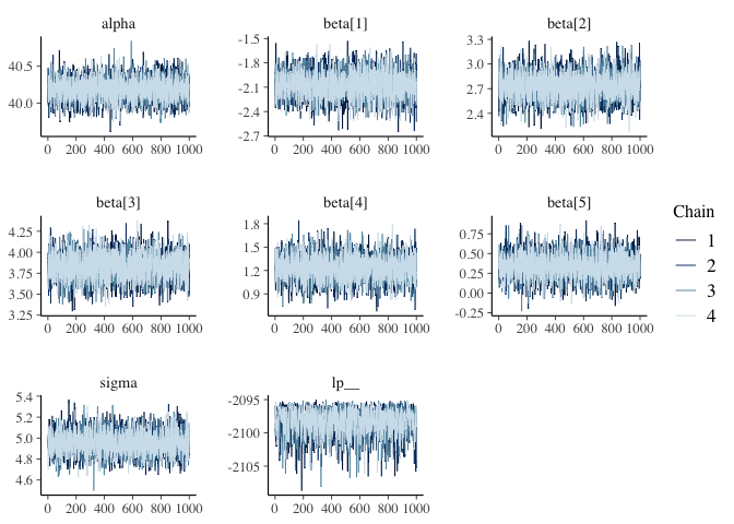
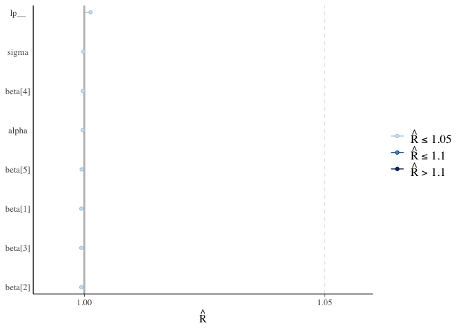
For Bayesian analysis, it is required to investigate the properties of the MCMC chains and the sampler in general, in addition to the standard model diagnostic checks (such as residual plots). Remember that the goal of MCMC sampling is to reproduce the posterior distribution of the model likelihood and priors by formulating a probability distribution. This method reliable, only if the MCMC samples accurately reflect the posterior. For each parameter, traceplots show the MCMC sample values after each iteration along the chain. Bad chain mixing (any pattern) indicates that the MCMC sample chains may not have spanned all aspects of the posterior distribution and that further iterations are needed to ensure that the distribution is accurately represented. Each parameter’s autocorrelation graphic shows the degree of correlation between MCMC samples separated by different lags. The degree of correlation between each MCMC sample and itself, for example, is represented by a lag of (obviously this will be a correlation of ). The MCMC samples should be independent in order to obtain unbiased parameter estimations (uncorrelated). For each parameter, the potential scale reduction factor (Rhat) statistic offers a measure of sampling efficiency/effectiveness. All values should, in theory, be less than 1, if the sampler has values of or greater than 1, it is likely that it was not particularly efficient or effective. A misspecified model or extremely unclear priors that lead to misspecified parameter space might lead to this. We should have looked at the convergence diagnostics before looking at the summaries. For the effects model, we utilise the package mcmcplots to generate density and trace graphs. It’s crucial to evaluate if the chains have converged when using MCMC to fit a model. To visually inspect MCMC diagnostics, we propose the bayesplot software. The bayesplot package includes routines for displaying MCMC diagnostics and supports model objects from both rstan and rstanarm. We’ll show how to make a trace plot with the mcmc_trace() function and a plot of Rhat values with the mcmc rhat() function. By printing the model fit, we can examine the parameters in the console. For each parameter, we derive posterior means, standard errors, and quantiles. n eff and Rhat are two other terms we use. These are the results of Stan’s engine’s exploration of the parameter space. For the time being, it’s enough to know that when Rhat is 1, everything is well.
fit_rstan %>%
  mcmc_trace()

fit_rstan %>%
  rhat() %>%
  mcmc_rhat() +
  yaxis_text()

Parting thoughts
To finish this post, I’d like to point out that the rstanarm package makes it possible to fit STAN models without having to write them down and instead using standard R syntax, such as that found in a glm(). So, what’s the point of learning all this STAN jargon? It depends: if you’re merely fitting “classical” models to your data with no fanfare, just use rstanarm; it’ll save you time and the models in this package are unquestionably better parametrized (i.e. faster) than the one I presented here. Learning STAN, on the other hand, is a good approach to get into a very flexible and strong language that will continue to evolve if you believe you will need to fit your own models one day. rstanarm is a package that acts as a user interface for Stan on the front end, and enables R users to create Bayesian models without needing to learn how to code in Stan. Using the standard formula and data, you can fit a model in rstanarm. If you want to use rstan to fit a different model type, you’ll have to code it yourself. The prefix stan_ precedes the model fitting functions and is followed by the model type. stan glm() and stan glmer() are two examples. A complete list of rstanarm functions can be found on Cran’s package guide.
Conclusions Summary
This tutorial provided only a quick overview of how to fit simple linear regression models with the Bayesian software STAN and the rstan library and how to get a collection of useful summaries from the models. This is just a taste of the many models that STAN can fit; in future postings, we’ll look at generalised linear models, as well as non-normal models with various link functions and hierarchical models. The STAN model as provided here is quite adaptable and able to accommodate datasets of various sizes. Although this may appear to be a more difficult technique than just fitting a linear model in a frequentist framework, the real benefits of Bayesian methods become apparent as the analysis becomes more sophisticated (which is often the case in real applications), the flexibility of Bayesian modelling makes it very simple to account for increasingly complicated models.
