Time series clustering
Introduction
As a typical form of dynamic data, time-series data, appears in a wide range of situations, including stock data, health data, and machine monitoring, to mention a few. They provide some difficult problems due to their high dimensionality, typically associated with time-series. More specifically, a time-series dataset can also have many values that change at the same time, in which case it is referred to as a multivariate time-series. There are various methods for altering time-series in order to minimize dimensionality, and most of them have to do with the representation of time-series.
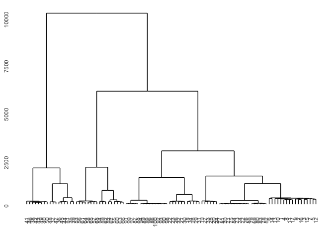
Cluster analysis is the process of categorising items into sets that are related to one another but as diverse from one another as possible. There are numerous strategies for performing clustering, and there is no uniform definition of a cluster. Every one of them outlines particular techniques to describe what a cluster is, how to calculate similarities, how to locate groupings quickly, etc. Series of time The most similar places in a space-time cube are found using a clustering tool, which divides them into separate clusters with members that share similar time series properties. Time series can be grouped according to how comparable their values are over time, how proportionate they remain over time, or how similar their smooth periodic patterns are over time. Time-series clustering is a type of clustering algorithm made to handle dynamic data. The most important elements to consider are the (dis)similarity or distance measure, the prototype extraction function, the clustering algorithm itself, and cluster evaluation. In many cases, algorithms developed for time-series clustering take static clustering algorithms and either modify the similarity definition, or the prototype extraction function to an appropriate one, or apply a transformation to the series so that static features are obtained. Therefore, the underlying basis for the different clustering procedures remains approximately the same across clustering methods. The most common approaches are hierarchical and partitional clustering, the latter of which includes fuzzy clustering.
Distance measures
- Euclidean distance
- most commonly used distance measure
- main limitations:
-
only for series of equal length
-
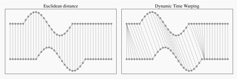
sensitive to time shifts
-
- Dynamic time warping (DTW) distance
-
shape based: can handle series with unequal length andovercomes Euclidean distance limitations
-
algorithm compares two series to find the optimum warping path
-
creates a local cost matrix and traverses it to find the optimal warping path
-
- main limitations:
-
choice of step pattern
-
choice of window that limits the area of the local cost matrix
-
computationally expensive
-
R packages
To the best of my knowledge, TSclust and dtwclust are the two main packages that perform time series clustering. These packages are incredibly straightforward yet effective time series analysis tools. Although the TSclust package provides a substantial amount of DTW functionality, it does not contain other methods that are extremely beneficial for time-series clustering. The implementation of new clustering algorithms like k-Shape and TADPole are in MATLAB, which makes it difficult to combine them with existing R programmes. The dtwclust package was created in order to connect with both established and emerging clustering methods while taking into account the uniqueness of time-series data. In this post we are going through the code for creating distance matrices, clustering, and visualizing the results using R.
First we load necessary packages and use the example example.database2.
suppressMessages(library(dplyr))
suppressMessages(library(TSdist))
suppressMessages(library(dtwclust))
suppressMessages(library(cluster))
suppressMessages(library(clusterCrit))
suppressMessages(library(TSclust))
suppressMessages(library(ggdendro))
data("example.database2")
Then lets visualize different data clusters.
N <- length(example.database2$classes)
labels <-  data.frame(key=1:N, label=example.database2$classes)
df <- t(example.database2$data) %>%
  as.data.frame() %>%
  `colnames<-`(1:N)

df %>%
  dplyr::mutate(t = 1:n()) %>%
  tidyr::gather(key, value, -t) %>%
  merge(labels) %>%
  ggplot2::ggplot()+
  ggplot2::geom_line(ggplot2::aes(x=t, y=value, group=key, color=label), alpha=0.5, show.legend = F)+
  ggplot2::facet_wrap(.~label)
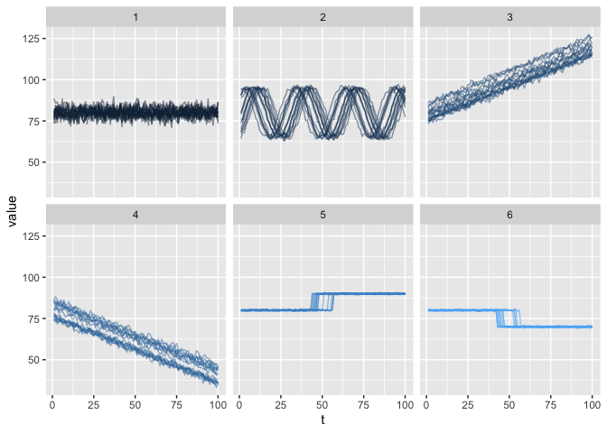
and to establish the (dis)symilarity between different clusters with an euclidean distance matrix.
diss <- TSdist::TSDatabaseDistances(example.database2$data, distance="euclidean", diag=T, upper=T) %>%
  as.matrix()
diss %>%
  reshape::melt() %>%
  ggplot2::ggplot()+
  ggplot2::geom_tile(ggplot2::aes(x = X1, y = X2, fill = value))+
  ggplot2::scale_fill_viridis_c()
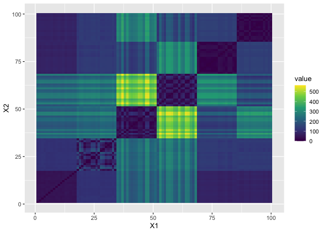
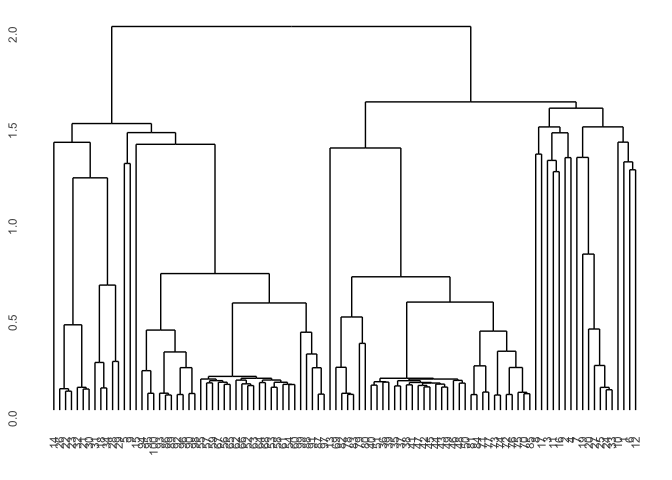
Now we take a look at different clustering procedures based on various (dis)symilarity measures. First let’s take a look at basic correlation based hierarchical clustering.
Diss1 <- diss(df, "COR")
hcl1 <- hclust(Diss1)
hcdata <- ggdendro::dendro_data(hcl1)
names_order <- hcdata$labels$label
p1 <- hcdata %>%
  ggdendro::ggdendrogram(., rotate=FALSE, leaf_labels=FALSE)
p1
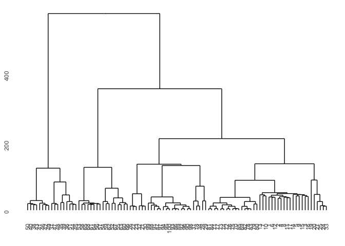
You can also simply change the distance measure in the diss function and for instance use the euclidean distance.
Diss2 <- diss(df, "EUCL")
hcl2 <- hclust(Diss2)
hcdata <- ggdendro::dendro_data(hcl2)
names_order <- hcdata$labels$label
p1 <- hcdata %>%
  ggdendro::ggdendrogram(., rotate=FALSE, leaf_labels=FALSE)
p1
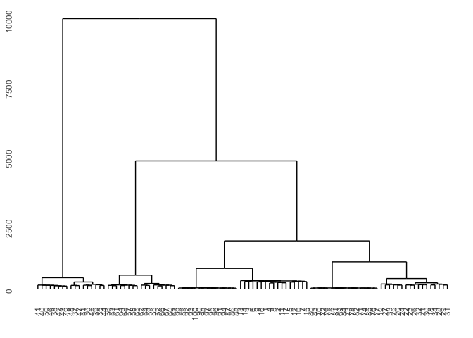
TSclust package provides DTWARP distance measures adapted for time series which can be used with hierarchical clustering.
dist_ts <- diss(SERIES = t(df), METHOD = "DTWARP")
hc <- hclust(dist_ts, method="complete")
hcdata <- dendro_data(hc)
names_order <- hcdata$labels$label
p1 <- hcdata %>%
  ggdendrogram(., rotate=FALSE, leaf_labels=FALSE)
p1
dtwclust package also provides DTWARP distance measures adapted for time series but with integrated clustering methods included.
dtwclust_ts <- tsclust(t(df),
                                    type = "h",
                                    k = 6,
                                    distance = "dtw",
                                    control = hierarchical_control(method = "complete"),
                                    preproc = NULL,
                                    args = tsclust_args(dist = list(window.size = 5L)))

hcdata <- dendro_data(dtwclust_ts)
names_order <- hcdata$labels$label
p1 <- hcdata %>%
  ggdendrogram(., rotate=FALSE, leaf_labels=FALSE)
p1
