Introduction: AutoML
Over the past few years, demand for machine learning systems has skyrocketed. This is mostly because machine learning techniques have been effective in a variety of applications. By enabling users from different backgrounds to apply machine learning models to address complicated scenarios, AutoML is fundamentally altering the face of ML-based solutions today. Nevertheless, despite abundant evidence that machine learning can benefit several industries, many firms today still find it difficult to implement ML models. This is due to a lack of seasoned and competent data scientists in the field. Additionally, many machine learning procedures call for more experience than knowledge, particularly when determining which models to train and how to evaluate them. Today, there are many efforts being made to close these gaps, which are rather obvious. We will examine in this post if AutoML can be a solution to these obstacles. Automated machine learning (AutoML) is the process of fully automating the machine learning application to practical issues. With the least amount of human effort, autoML aims to automate as many processes as possible in an ML pipeline without sacrificing the model’s performance. The training, fine-tuning, and deployment of machine learning models are all automated using the automated machine learning technique known as AutoML. Without the need for human participation, AutoML can be used to automatically find the optimal model for a particular dataset and task.
Because it can automate the process of developing and deploying machine learning models, AutoML is a crucial tool for making machine learning approachable to non-experts. This can expedite machine learning research and save time and resources. The key innovation in AutoML is the hyperparameters search technique, which is used for preprocessing elements, choosing model types, and improving their hyperparameters. There are many different types of optimization algorithms, ranging from Bayesian and evolutionary algorithms to random and grid search. Various strategies can be used to develope an AutoML solution, depending on the precise issue that has to be resolved. For instance, some approaches concentrate on identifying the best model for a particular job, while others concentrate on optimising a model for a specific dataset. Whatever the strategy, AutoML can be a potent tool for improving the usability and effectiveness of machine learning.
This post aims to introduce you to H2O as one of the top AutoML Tools and Platforms.
Pro’s
-
Time saving: It’s a quick prototyping tool, specially if you are not working on critical task, you could use AutoML to do the job for you while you focus on more critical tasks.
-
Benchmarking: Building a ML/DL model is fun, but, how to know if the model is the best? One option is to use AutoML to benchmark yours.
Con’s
-
Most AI models that we come across are black box. Similar is the case with these AutoML frameworks. If you don’t understand what you are doing, it could be catastrophic.
-
Based on the previous point, AutoML is being marketed as a tool for non-data scientists. However, without understanding how a model works and blindly using it for making decisions could be disastrous.
H2O AutoML
The AutoML component of the H2O packahe enables the automatic training and fine-tuning of several models within a user-specified time frame. Using all of the models, the current AutoML function can train and cross-validate a Random Forest, an Extremely-Randomized Forest, a random grid of Gradient Boosting Machines (GBMs), a random grid of Deep Neural Nets, and a Stacked Ensemble. In order for users to complete jobs with the least amount of misunderstanding, AutoML should take into account the issues of data preparation, model development, and ensembles while also offering as few parameters as feasible. With only a few user-supplied parameters, H2O AutoML is able to complete this work with simplicity. The data-related arguments x, y, training frame, and validation frame are used in both the R and Python APIs; y and training frame are required parameters, and the rest are optional. Max runtime sec is a necessary parameter, while max model is optional; if you don’t supply any parameters, it defaults to taking NULL. You may also adjust values for these parameters here. If you don’t want to use every predictor from the frame you gave, you can set it by supplying it to the x parameter, which is the vector of predictors from training frame. Now let’s discuss a few optional and unrelated parameters; try to adjust the settings even if you are unaware of their purpose; doing so will help you learn about some complex subjects:
-
Enter a dataframe (df) and select the independent variable (y) that you want to forecast. If you want to ensure that your results can be replicated, you can set or modify the seed argument.
-
The function determines whether the model is a classification (categorical) or regression (continuous) model by examining the class and number of distinct values of the independent variable (y), which can be adjusted using the thresh parameter.
-
Test and train datasets will be separated from the dataframe. With the split argument, the split percentage can be managed. The msplit() function can duplicate this.
-
Before moving on, you could also scale and centre your numerical data, use the no outliers function to remove some outliers, and/or use MICE to impute missing values. The function can balance (under-sample) your training data if the model is a classification model. This behaviour is manageable using the balance argument. Up until this point, the model preprocess() function can be used to duplicate the entire procedure.
-
Runs h2o::h2o.automl(…) to train several models and provide a leaderboard of the best (max models or max time) trained models, ranked by effectiveness. You can also modify certain extra arguments you want to provide to the mother function, such as nfolds for k-fold cross-validations, exclude algos and include algos to exclude or include particular algorithms, and any other extra argument you want.
-
The best model, given the default performance metric (which can be modified with the stopping metric option), will be chosen to proceed after being cross-validated and evaluated using nfolds. A different model can be chosen using the h2o selectmodel() method, and all calculations and plots can then be redone using this new model.
-
The test predictions and test actual values will be used to create and render performance metrics and charts (which were NOT passed to the models as inputs to be trained with). Your model’s performance metrics shouldn’t be skewed in this way. The model metrics() method lets you repeat these calculations.
-
A list containing all the inputs, performance metrics, graphs, the top-ranked model, and leaderboard results. The results can be exported by using the export results() function, or you can (play) see them on the console.
Mapping H2O AutoML Functionalities
-
Validation_frame: This parameter is used for early stopping of individual models in the automl. It is a dataframe that you pass for validation of a model or can be a part of training data if not passed by you.
-
leaderboard_frame: If passed the models will be scored according to the values instead of using cross-validation metrics. Again the values are a part of training data if not passed by you.
-
nfolds: K-fold cross-validation by default 5, can be used to decrease the model performance.
-
fold_columns: Specifies the index for cross-validation.
-
All three frames are passed - No splits.
-
Only training frame is passed - The data is split into 80/10/10 training, validation, and leaderboard.
-
Training and leaderboard frame is passed - Data split into 80-20 of training and validation frames.
-
-
Weights_column: If you want to provide weights to specific columns you can use this parameter, assigning weight 0 means you are excluding the column. ignored_columns: Only in python, it is converse of x.
-
Stopping_metric: Specifies a metric for early stopping of the grid searches and models default value is logloss for classification and deviation for regression.
-
Sort_metric: The parameter to sort the leaderboard models at the end. This defaults to AUC for binary classification, mean_per_class_error for multinomial classification, and deviance for regression.
-
The validation_frame and leaderboard_frame depend on the cross-validation parameter that is nfolds.
H2O AutoML satisfies the need for machine learning experts by developing intuitive machine learning software. This AutoML application seeks to streamline machine learning by offering clear and uniform user interfaces for different machine learning methods. Within a user-specified time range, machine learning models are automatically developed and fine-tuned. The lares package contains several families of functions that enable data scientists and analysts to perform high-quality, reliable analyses without having to write a lot of code. H2O automl, which semi-automatically executes the entire pipeline of a Machine Learning model given a dataset and some adjustable parameters, is one of our more intricate yet valuable functions. You can speed up research and development by using AutoML to train high-quality models that are tailored to your needs.
Before getting to the code, I recommend checking h2o_automl’s full documentation here or within your R session by running ?lares::h2o_automl if you use the lares version. Documentation contains a brief explanation of each parameter that can be entered into the function to acquire the results you need and regulate how it operates.
first we load the necessay packages
library(readr)
library(tidyverse)
library(tidymodels)
library(h2o)
library(gridExtra)
library(kableExtra)
we use the diabetes data from pdp package
data(pima, package = "pdp")
out="diabetes"
preds=colnames(pima)[-c(9)]
df=pima%>%
  drop_na()

df_split <- initial_split(df)
train_data <- training(df_split)
test_data <- testing(df_split)
h2o.init()
train_data <- as.h2o(train_data)
here we train the model
h2oAML <- h2o.automl(
  y = out,
  x = preds,
  training_frame = train_data,
  project_name = "ice_the_kicker_bakeoff",
  balance_classes = T,
  max_runtime_secs = 100,
  seed = 1234
)
a summary can be found in the leaderboard_tbl object
leaderboard_tbl <- h2oAML@leaderboard %>% as_tibble()

leaderboard_tbl %>% head() %>% kable()
| model_id | auc | logloss | aucpr | mean_per_class_error | rmse | mse |
|---|---|---|---|---|---|---|
| GBM_grid_1_AutoML_1_20221024_112632_model_40 | 0.8475490 | 0.4392863 | 0.6840091 | 0.1936275 | 0.3764929 | 0.1417469 |
| StackedEnsemble_BestOfFamily_7_AutoML_1_20221024_112632 | 0.8446623 | 0.4507552 | 0.6834712 | 0.1915033 | 0.3765024 | 0.1417541 |
| GBM_grid_1_AutoML_1_20221024_112632_model_30 | 0.8435185 | 0.4571160 | 0.7007188 | 0.1918301 | 0.3830612 | 0.1467359 |
| DeepLearning_grid_1_AutoML_1_20221024_112632_model_3 | 0.8424837 | 0.4846210 | 0.6730490 | 0.2058824 | 0.3863806 | 0.1492899 |
| GBM_grid_1_AutoML_1_20221024_112632_model_87 | 0.8423203 | 0.4560024 | 0.6421818 | 0.2081699 | 0.3858873 | 0.1489090 |
| StackedEnsemble_AllModels_6_AutoML_1_20221024_112632 | 0.8414488 | 0.4586412 | 0.6550735 | 0.1942810 | 0.3806513 | 0.1448954 |
the leaderboard_tbl object also alows us to identify the best fitting model
model_names <- leaderboard_tbl$model_id

top_model <- h2o.getModel(model_names[1])

top_model@model$model_summary %>%pivot_longer(cols = everything(),names_to = "Parameter", values_to = "Value") %>%kable()
| Parameter | Value |
|---|---|
| number_of_trees | 36.000000 |
| number_of_internal_trees | 36.000000 |
| model_size_in_bytes | 4499.000000 |
| min_depth | 3.000000 |
| max_depth | 5.000000 |
| mean_depth | 3.638889 |
| min_leaves | 4.000000 |
| max_leaves | 6.000000 |
| mean_leaves | 5.305555 |
then we can measure the performance on the test data
h2o_predictions <- h2o.predict(top_model, newdata = as.h2o(test_data)) %>%
  as_tibble() %>%
  bind_cols(test_data)
h2o_metrics <- bind_rows(
  #Calculate Performance Metrics
  yardstick::f_meas(h2o_predictions, diabetes, predict),
  yardstick::precision(h2o_predictions, diabetes, predict),
  yardstick::recall(h2o_predictions, diabetes, predict)
) %>%
  mutate(label = "h2o", .before = 1) %>%
  rename_with(~str_remove(.x, '\\.'))  %>% kable()
here is the code to make the confusion matrix on the test data
h2o_cf <- h2o_predictions %>%
  count(diabetes, pred= predict) %>%
  mutate(label = "h2o", .before = 1)%>% kable()
Lares package provides an elegant wrapper for H2O AutoML functions
library(lares)

r <- h2o_automl( train_data, y = diabetes, max_models = 10, impute = FALSE, target = 'pos')
you can extract feature importance
head(r$importance)%>% kable()
| variable | relative_importance | scaled_importance | importance |
|---|---|---|---|
| glucose | 46.2070580 | 1.0000000 | 0.4943360 |
| age | 21.4305954 | 0.4637948 | 0.2292705 |
| insulin | 14.2493601 | 0.3083806 | 0.1524436 |
| triceps | 6.5016131 | 0.1407061 | 0.0695561 |
| pedigree | 5.0137486 | 0.1085061 | 0.0536385 |
| mass | 0.0706036 | 0.0015280 | 0.0007553 |
metrics for the perforamnce
r$metrics %>% kable()
|
|
|
|
|
|
A general plot of the performance as follows :
plot(r)
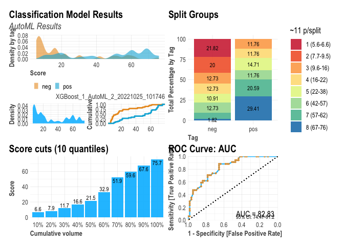
as well as specific plots.
r$plots$metrics
## $gains
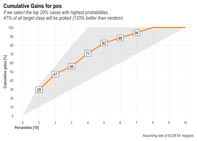
##
## $response
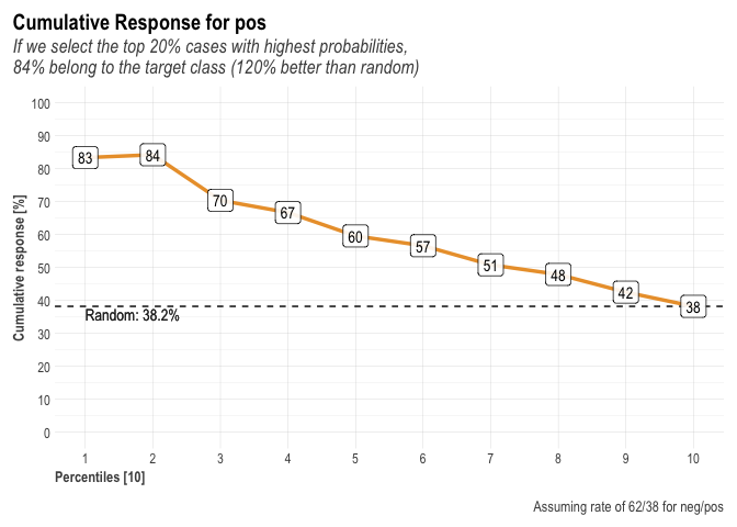
##
## $conf_matrix
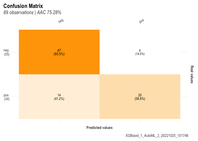
##
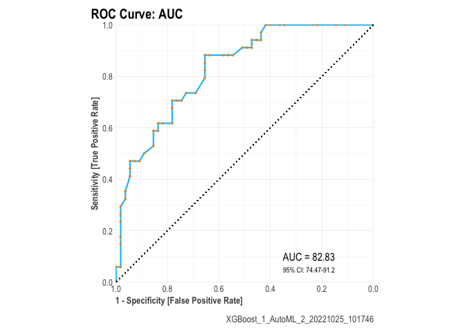
## $ROC
