Bayesian Multilevel models in brms
Multilevel models (MLMs)
Multilevel models (MLMs) offer great flexibility for researchers allow modeling of data measured on different levels (e.g. data of students nested within classes and schools) thus taking complex dependency structures into account. This is done by fitting models that include both constant and varying effects (sometimes referred to as fixed and random effects). The multilevel strategy can be especially useful when dealing with repeated measurements (e.g., when measurements are nested within participants) or when handling complex dependency structures in the data such as unequal sample sizes. Many R packages are developed to fit MLMs with their functionality of limited to the mean of the response distribution while other parameters of the response distribution, such as the residual standard deviation in linear models, are assumed constant across observations. However, when one tries to include the maximal varying effect structure, this kind of model tends either not to converge, or to give aberrant estimations of the correlation between varying effects, however, the maximal varying effect structure can generally be fitted in a Bayesian framework. Another advantage of Bayesian statistical modelling is that it fits the way researchers intuitively understand statistical results. Widespread misinterpretations of frequentist statistics (like p-values and confidence intervals) are often attributable to the wrong interpretation of these statistics as resulting from a Bayesian analysis. The intuitive nature of the Bayesian approach might arguably be hidden by the predominance of frequentist teaching in undergraduate statistical courses. Moreover, the Bayesian approach offers a natural solution to the problem of multiple comparisons, when the situation is adequately modelled in a multilevel framework, and allows a priori knowledge to be incorporated in data analysis via the prior distribution. In this post, we will briefly introduce the Bayesian approach to data analysis and the multilevel modelling strategy. Second, we will illustrate how Bayesian MLMs can be implemented in R by using the brms package.
Bayesian Method
The key difference between Bayesian statistical inference and frequentist statistical methods concerns the nature of the unknown parameters to be estimated. In the frequentist framework, a parameter of interest is assumed to be unknown, but fixed. That is, it is assumed that in the population there is only one true population parameter, for example, one true mean or one true regression coefficient. In the Bayesian view of subjective probability, all unknown parameters are treated as uncertain and therefore are be described by a probability distribution. Every parameter is unknown, and everything unknown receives a distribution. This post first build towards a full multilevel using uninformative priors and then will discuss the influence of using different priors on the final model. If you’re just starting out with Bayesian statistics in R and you have some familiarity with running Frequentist models using packages like lme4 or the base lm function, you may prefer starting out with more user-friendly packages that use Stan as a backend, but hide a lot of the complicated details. brms package gives us the actual posterior samples, lets us specify a wide range of priors, and using the familiar input structure of the lme4 package. As presented in previous posts Stan is the way to go if you want more control and a deeper understanding of your models. Stan comes with its own programming language, allowing for great modeling flexibility. Many researchers may still be hesitent to use Stan directly, as every model has to be written, debugged and possibly also optimized. This may be a time-consuming and error-prone process even for researchers familiar with Bayesian inference. The brms package, presented here, allows the user to benefit from the merits of Stan by using extended lme4-like formula syntax, with which many R users are familiar with. It offers much more than writing efficient and human-readable Stan code. brms comes with many post-processing and visualization functions, for instance to perform posterior predictive checks, leave one-out cross-validation, visualization of estimated effects, and prediction of new data. Since the brms package (via STAN) makes use of a Hamiltonian Monte Carlo sampler algorithm (MCMC) to approximate the posterior (distribution), we need to specify a few more parameters than in a frequentist analysis (using lme4).
- First we need the specify the number of iterations.
- We need to specify the number of chains.
- We need to specify the number of iterations per chain (warmup or burnin phase).
- We need to specify initial values are for the different chains for the parameters of interest.
We need to specify all these values for replicability purposes. In addition, if the two chains would not converge we can specify more iterations, different starting values and a longer warmup period.
The brm() function requires:
- the dependent variable to predict.
- a “~”, to indicate that we now give the other variables of interest.
- a “1” in the formula the function indicates the intercept.
-
the random effects/slopes between brackets. Again the value 1 is to indicate the intercept and the variables right of the vertical “ ” bar is used to indicate grouping variables. - Finally, we specify which dataset we want to use after the data = dataset.
Here is an example:
lmm.data <- read.table("http://bayes.acs.unt.edu:8083/BayesContent/class/Jon/R_SC/Module9/lmm.data.txt",
                       header=TRUE, sep=",", na.strings="NA", dec=".", strip.white=TRUE)
#summary(lmm.data)
head(lmm.data)
model0 <- brm(extro ~ 1 + (1|school),
              data = lmm.data,
              warmup = 1000, iter = 5000,
              cores = 4, chains = 4,
              seed = 123) #to run the model
summary(model0)
##  Family: gaussian
##   Links: mu = identity; sigma = identity
## Formula: extro ~ 1 + (1 | school)
##    Data: lmm.data (Number of observations: 1200)
##   Draws: 4 chains, each with iter = 5000; warmup = 1000; thin = 1;
##          total post-warmup draws = 16000
##
## Group-Level Effects:
## ~school (Number of levels: 6)
##               Estimate Est.Error l-95% CI u-95% CI Rhat Bulk_ESS Tail_ESS
## sd(Intercept)    10.53      3.32     6.04    18.82 1.00     2921     3976
##
## Population-Level Effects:
##           Estimate Est.Error l-95% CI u-95% CI Rhat Bulk_ESS Tail_ESS
## Intercept    60.45      3.87    52.85    68.15 1.00     2498     3429
##
## Family Specific Parameters:
##       Estimate Est.Error l-95% CI u-95% CI Rhat Bulk_ESS Tail_ESS
## sigma     2.67      0.05     2.57     2.78 1.00     5357     6299
##
## Draws were sampled using sampling(NUTS). For each parameter, Bulk_ESS
## and Tail_ESS are effective sample size measures, and Rhat is the potential
## scale reduction factor on split chains (at convergence, Rhat = 1).
model1 <- brm(extro ~ open + agree + social + (1|school),
              data = lmm.data,
              warmup = 1000, iter = 5000,
              cores = 4, chains = 4,
              seed = 123) #to run the model
summary(model1)
##  Family: gaussian
##   Links: mu = identity; sigma = identity
## Formula: extro ~ open + agree + social + (1 | school)
##    Data: lmm.data (Number of observations: 1200)
##   Draws: 4 chains, each with iter = 5000; warmup = 1000; thin = 1;
##          total post-warmup draws = 16000
##
## Group-Level Effects:
## ~school (Number of levels: 6)
##               Estimate Est.Error l-95% CI u-95% CI Rhat Bulk_ESS Tail_ESS
## sd(Intercept)    10.65      3.45     6.15    19.29 1.00     4871     6925
##
## Population-Level Effects:
##           Estimate Est.Error l-95% CI u-95% CI Rhat Bulk_ESS Tail_ESS
## Intercept    59.11      4.10    50.88    67.40 1.00     3389     5129
## open          0.01      0.01    -0.02     0.04 1.00    15266     9414
## agree         0.03      0.02    -0.00     0.06 1.00    15431     9360
## social       -0.00      0.00    -0.01     0.01 1.00    18096     9605
##
## Family Specific Parameters:
##       Estimate Est.Error l-95% CI u-95% CI Rhat Bulk_ESS Tail_ESS
## sigma     2.67      0.05     2.57     2.78 1.00    15687     9773
##
## Draws were sampled using sampling(NUTS). For each parameter, Bulk_ESS
## and Tail_ESS are effective sample size measures, and Rhat is the potential
## scale reduction factor on split chains (at convergence, Rhat = 1).
model2 <- brm(extro ~ open + agree + social + (1 + social |school),
              data = lmm.data,
              warmup = 1000, iter = 5000,
              cores = 4, chains = 4,
              seed = 123) #to run the model
summary(model2)
##  Family: gaussian
##   Links: mu = identity; sigma = identity
## Formula: extro ~ open + agree + social + (1 + social | school)
##    Data: lmm.data (Number of observations: 1200)
##   Draws: 4 chains, each with iter = 5000; warmup = 1000; thin = 1;
##          total post-warmup draws = 16000
##
## Group-Level Effects:
## ~school (Number of levels: 6)
##                       Estimate Est.Error l-95% CI u-95% CI Rhat Bulk_ESS
## sd(Intercept)            10.44      3.40     5.83    18.88 1.00     5639
## sd(social)                0.01      0.01     0.00     0.04 1.00     4468
## cor(Intercept,social)     0.33      0.46    -0.68     0.97 1.00    10247
##                       Tail_ESS
## sd(Intercept)             9050
## sd(social)                5332
## cor(Intercept,social)     8834
##
## Population-Level Effects:
##           Estimate Est.Error l-95% CI u-95% CI Rhat Bulk_ESS Tail_ESS
## Intercept    59.16      3.92    51.38    66.93 1.00     3440     5465
## open          0.01      0.01    -0.02     0.04 1.00    23467    10482
## agree         0.03      0.02    -0.00     0.06 1.00    23836    10931
## social       -0.00      0.01    -0.02     0.02 1.00     8721     7519
##
## Family Specific Parameters:
##       Estimate Est.Error l-95% CI u-95% CI Rhat Bulk_ESS Tail_ESS
## sigma     2.67      0.05     2.57     2.78 1.00    23299    11201
##
## Draws were sampled using sampling(NUTS). For each parameter, Bulk_ESS
## and Tail_ESS are effective sample size measures, and Rhat is the potential
## scale reduction factor on split chains (at convergence, Rhat = 1).
Priors
As stated in the brms manual: “Prior specifications are flexible and explicitly encourage users to apply prior distributions that actually reflect their beliefs.” Here we will only focus on priors for the regression coefficients and not on the error and variance terms, since we are most likely to actually have information on the size and direction of a certain effect and less (but not completely) unlikely to have prior knowledge on the unexplained variances.
get_prior(extro ~ open + agree + social + (1 + social |school), data = lmm.data)
                  prior     class      coef  group resp dpar nlpar lb ub       source
                  (flat)         b                                             default
                  (flat)         b     agree                              (vectorized)
                  (flat)         b      open                              (vectorized)
                  (flat)         b    social                              (vectorized)
                  lkj(1)       cor                                             default
                  lkj(1)       cor           school                       (vectorized)
 student_t(3, 60.2, 9.2) Intercept                                             default
    student_t(3, 0, 9.2)        sd                                   0         default
    student_t(3, 0, 9.2)        sd           school                  0    (vectorized)
    student_t(3, 0, 9.2)        sd Intercept school                  0    (vectorized)
    student_t(3, 0, 9.2)        sd    social school                  0    (vectorized)
    student_t(3, 0, 9.2)     sigma                                   0         default
prior1 <- c(set_prior("normal(0,10)", class = "b", coef = "open"),
            set_prior("normal(0,10)", class = "b", coef = "agree"),
            set_prior("normal(0,10)", class = "b", coef = "social"))
modelp <- brm(extro ~ open + agree + social + (1|school),
              data = lmm.data,
              prior = prior1,
              warmup = 1000, iter = 5000,
              cores = 4, chains = 4,
              seed = 123)
summary(modelp)
##  Family: gaussian
##   Links: mu = identity; sigma = identity
## Formula: extro ~ open + agree + social + (1 | school)
##    Data: lmm.data (Number of observations: 1200)
##   Draws: 4 chains, each with iter = 5000; warmup = 1000; thin = 1;
##          total post-warmup draws = 16000
##
## Group-Level Effects:
## ~school (Number of levels: 6)
##               Estimate Est.Error l-95% CI u-95% CI Rhat Bulk_ESS Tail_ESS
## sd(Intercept)    10.56      3.41     6.06    19.15 1.00     4393     7131
##
## Population-Level Effects:
##           Estimate Est.Error l-95% CI u-95% CI Rhat Bulk_ESS Tail_ESS
## Intercept    59.05      3.95    51.30    67.00 1.00     3631     5299
## open          0.01      0.01    -0.02     0.04 1.00    15390    10073
## agree         0.03      0.02    -0.00     0.06 1.00    15738    10121
## social       -0.00      0.00    -0.01     0.01 1.00    18386    10795
##
## Family Specific Parameters:
##       Estimate Est.Error l-95% CI u-95% CI Rhat Bulk_ESS Tail_ESS
## sigma     2.67      0.05     2.57     2.78 1.00    13509     9902
##
## Draws were sampled using sampling(NUTS). For each parameter, Bulk_ESS
## and Tail_ESS are effective sample size measures, and Rhat is the potential
## scale reduction factor on split chains (at convergence, Rhat = 1).
Trace-plots and convergence dianostics
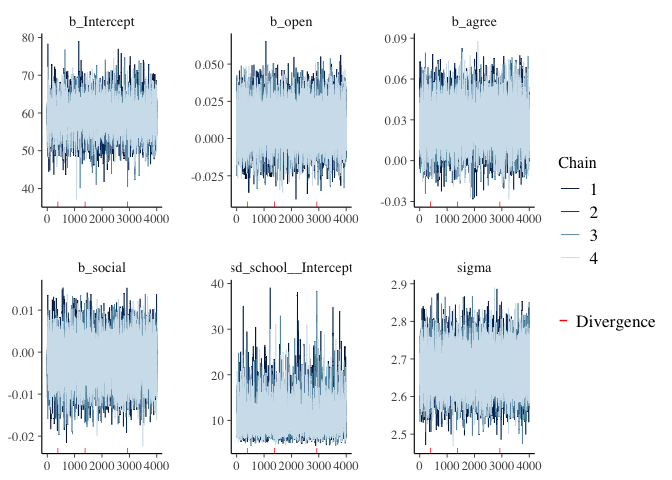
Before interpreting results, we should inspect the convergence of the chains that form the posterior distribution of the model parameters. A straightforward and common way to visualize convergence is the trace plot that illustrates the iterations of the chains from start to end.
mcmc_plot(model1, type = "trace")

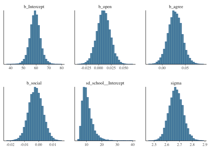
mcmc_plot(model1, type = "hist")

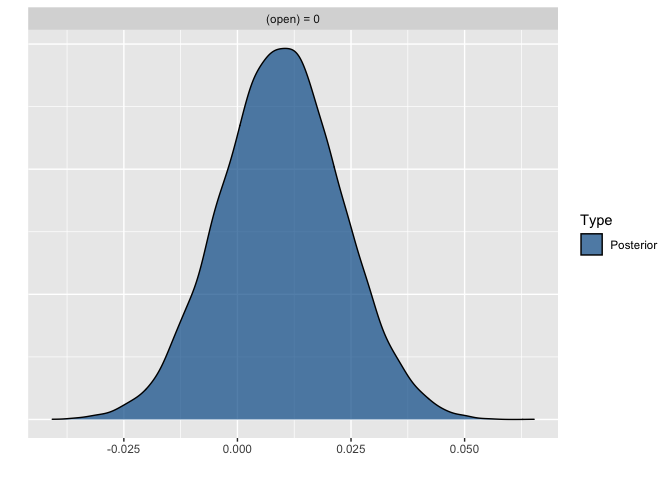
plot(hypothesis(model1, "open = 0"))

Conclusion
This post is meant to introduce users to the flexibility of the distributional regression approach and corresponding formula syntax as implemented in brms and fitted with Stan behind the scenes. Only a subset of modeling options were discussed in detail. Many more examples can be found in the growing number of vignettes accompanying the package (see vignette(package = “brms”) for an overview). To date, brms is already one of the most flexible R packages when it comes to regression modeling.
