Partially Observable Markov Decision Process (POMDP) in R
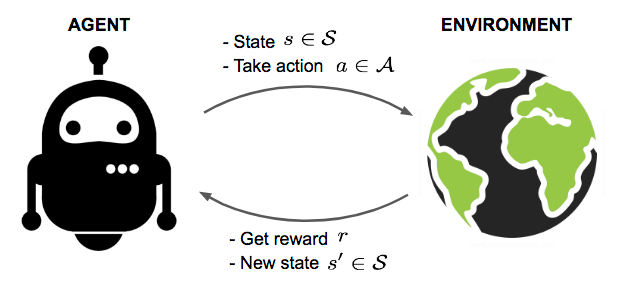
A Markov Decision Process (MDP) provides a principled mathematical framework for sequential decision-making under uncertainty, in which an agent selects actions based on a fully observed system state. A Partially Observable Markov Decision Process (POMDP) generalizes this framework to settings in which the true system state is not directly accessible to the agent. Formally, a POMDP is defined by the tuple $\langle S, A, \Omega, T, O, R, \gamma \rangle$, where $S$ is the state space, $A$ is the action space, $\Omega$ is the observation space, $T: S \times A \times S \to [0,1]$ is the transition model, $O: S \times A \times \Omega \to [0,1]$ is the observation model, $R: S \times A \to \mathbb{R}$ is the reward function, and $\gamma \in [0,1]$ is the discount factor.
Because the agent cannot directly observe $s \in S$, it maintains a belief state $b \in \Delta(S)$ — a probability distribution over all possible states — which is updated via Bayesian inference upon receiving each observation. The policy function $\pi: \Delta(S) \to A$ maps belief states to actions, in contrast to the MDP case where $\pi: S \to A$. The objective is to identify an optimal policy $\pi^*$ that maximises the expected discounted cumulative reward:
\[V^{\pi^*}(b_0) = \max_{\pi} \mathbb{E}\left[\sum_{t=0}^{\infty} \gamma^t R(s_t, a_t) \,\Big|\, b_0, \pi \right]\]Partial observability arises from two principal sources. First, multiple distinct states may produce identical perceptual readings, a phenomenon known as perceptual aliasing, in which different regions of the environment appear indistinguishable to the agent’s perceptual system yet require different actions. Second, perceptual noise may cause the same state to yield varying observations across successive time steps. The POMDP captures both sources of uncertainty through the probabilistic observation model $O(o \mid s’, a)$, which specifies the conditional likelihood of receiving observation $o \in \Omega$ after transitioning to state $s’ \in S$ under action $a \in A$.
Belief state updating follows Bayes’ rule. After taking action $a$ and observing $o$, the posterior belief is:
\[b'(s') = \eta \cdot O(o \mid s', a) \sum_{s \in S} T(s' \mid s, a)\, b(s)\]where $\eta$ is a normalising constant ensuring $\sum_{s’} b’(s’) = 1$. The POMDP framework subsumes a Hidden Markov Model (HMM) — which characterises stochastic state transitions and probabilistic observations — within an MDP that governs action selection and reward accumulation. Exact POMDP solutions are computationally intractable for large state spaces, as the belief state is continuous and the resulting value function is defined over a continuous simplex. However, it can be shown that the optimal value function $V^*(b)$ is piecewise linear and convex (PWLC) in the belief state, which underlies the family of point-based approximate solvers widely used in practice.
Applications of POMDPs span robot navigation, medical decision-making,
machine maintenance, and computational psychiatry. Despite their broad
applicability, POMDPs remain underutilised in many domains, partly due
to the mathematical complexity of exact and approximate solvers and the
relative scarcity of accessible implementation resources. This post
provides a rigorous introduction to POMDPs and demonstrates their
specification and solution in R using the pomdp package.
Package Overview
Solving a POMDP problem with the pomdp package consists of two steps:
- Define the POMDP model using the
POMDP()constructor function. - Solve the model using
solve_POMDP().
Defining a POMDP Model
The POMDP() function accepts the following arguments, each
corresponding to a formal element of the POMDP tuple:
str(args(POMDP))
states— defines the finite state space $S = {s_1, s_2, \ldots, s_n}$actions— defines the finite action space $A = {a_1, a_2, \ldots, a_k}$observations— defines the finite observation space $\Omega = {o_1, o_2, \ldots, o_m}$transition_prob— specifies the conditional transition probabilities $T(s’ \mid s, a) = \Pr(s_{t+1} = s’ \mid s_t = s,\, a_t = a)$observation_prob— specifies the conditional observation probabilities $O(o \mid s’, a) = \Pr(o_t = o \mid s_t = s’,\, a_{t-1} = a)$reward— specifies the reward function $R(s, a)$ or $R(s, a, s’, o)$discount— the discount factor $\gamma \in [0, 1]$, controlling the trade-off between immediate and long-term rewardhorizon— the planning horizon $H$; set toInffor the infinite-horizon formulationterminal_values— a vector of state utilities $V_H(s)$ applied at the terminal time stepstart— the initial belief state $b_0$, specified as a probability distribution over $S$max— logical flag indicating whether the objective is reward maximisation or cost minimisationname— an identifying label for the POMDP instance
Solving a POMDP
POMDP problems are solved via solve_POMDP(). The full list of solver
parameters is available through solve_POMDP_parameter(); detailed
documentation appears in the solve_POMDP() manual page.
str(args(solve_POMDP))
horizon— specifies the finite planning horizon $H$ (number of decision epochs). When set toNULL, the solver iterates until convergence to the infinite-horizon solution.method— selects the solution algorithm. Available methods include"grid"(grid-based value iteration),"enum"(exhaustive enumeration),"twopass","witness", and"incprune"(incremental pruning). Additional solver hyperparameters are passed as a named list via theparametersargument.
Applied Example: Mood Updating Under Partial Observability
The following example implements the POMDP model from Clark & Watson (2023), Modelling mood updating: a proof of principle study, a computational psychiatry study examining how a healthy agent updates beliefs about environmental valence under conditions of partial observability.
The POMDP components are specified as follows:
- $S = {\texttt{Stressful},\, \texttt{Not-Stressful}}$: the set of latent environmental states, representing the affective valence of the current context.
- $A = {\texttt{Wait},\, \texttt{amplify-stress-signals},\, \texttt{attenuate-stress-signals},\, \texttt{amplify-pleasure-signals},\, \texttt{attenuate-pleasure-signals}}$: the action space encoding the agent’s attentional and regulatory strategies.
- $T(s’ \mid s, a)$: a state-dependent transition matrix encoding prior beliefs about how each action preserves or shifts the latent state. Values were chosen to reflect a healthy agent’s belief that deliberate attentional actions reliably preserve the current state.
- $R(s, a) = -\log P(\text{outcome} \mid T)$: reward is defined as the surprisal — the negative log-probability — of the resulting state given the agent’s prior beliefs under action $a$. This formulation operationalises the free-energy minimisation principle: the agent selects actions that minimise prediction error.
- $\Omega = {\texttt{Stress-Signals},\, \texttt{Pleasure-Signals}}$: the set of observable signals available to the agent.
- $O(o \mid s’, a)$: a conditional observation matrix encoding prior beliefs about which signals are likely given the latent state and selected action.
- $\gamma = 0.5$: the discount factor, set at an intermediate value reflecting a balance between immediate and future prediction error minimisation. As noted by the authors, emerging evidence implicates the discount factor in pathological mood states.
Transition Probability Matrix $T(s’ \mid s, a)$
The matrix a encodes $T(s’ \mid s, a)$ for each action. Parameter
values were chosen to reflect the healthy agent’s prior certainty that
actions will reliably sustain the current belief state. For instance,
amplifying stress signals is associated with a 90% probability that the
environment remains in the stressful state. The "identity"
specification for the Wait action denotes that passive waiting leaves
the state distribution unchanged.
library(pomdp)

a <- list(
  "Wait" = "identity",
  "amplify-stress-signals"    = matrix(c(0.9, 0.1, 0.6, 0.4), nrow = 2, byrow = TRUE),
  "attenuate-stress-signals"  = matrix(c(0.4, 0.6, 0.25, 0.75), nrow = 2, byrow = TRUE),
  "amplify-pleasure-signals"  = matrix(c(0.25, 0.75, 0.1, 0.9), nrow = 2, byrow = TRUE),
  "attenuate-pleasure-signals"= matrix(c(0.75, 0.25, 0.6, 0.4), nrow = 2, byrow = TRUE)
)
Each $2 \times 2$ matrix entry $T_{ij}$ gives $\Pr(s_{t+1} = s_j \mid s_t = s_i, a)$, with rows corresponding to the current state and columns to the successor state ($s_1 = \texttt{Stressful}$, $s_2 = \texttt{Not-Stressful}$):
|
|
|
|
|
Observation Probability Matrix $O(o \mid s’, a)$
The matrix b encodes $O(o \mid s’, a)$, the conditional probability of
observing signal $o$ given that the system transitioned to state $s’$
under action $a$. These values reflect strong prior beliefs that
observed signals are congruent with their corresponding latent states —
e.g., a stressful state following stress amplification yields a stress
signal with probability 0.9.
b <- rbind(
  O_("amplify-stress-signals",    "Stressful",     "Stress-Signals",   0.9),
  O_("amplify-stress-signals",    "Not-Stressful", "Stress-Signals",   0.3),
  O_("amplify-stress-signals",    "Stressful",     "Pleasure-Signals", 0.1),
  O_("amplify-stress-signals",    "Not-Stressful", "Pleasure-Signals", 0.7),
  O_("attenuate-stress-signals",  "Stressful",     "Stress-Signals",   0.6),
  O_("attenuate-stress-signals",  "Not-Stressful", "Stress-Signals",   0.1),
  O_("attenuate-stress-signals",  "Stressful",     "Pleasure-Signals", 0.4),
  O_("attenuate-stress-signals",  "Not-Stressful", "Pleasure-Signals", 0.9),
  O_("amplify-pleasure-signals",  "Stressful",     "Stress-Signals",   0.6),
  O_("amplify-pleasure-signals",  "Not-Stressful", "Stress-Signals",   0.1),
  O_("amplify-pleasure-signals",  "Stressful",     "Pleasure-Signals", 0.4),
  O_("amplify-pleasure-signals",  "Not-Stressful", "Pleasure-Signals", 0.9),
  O_("attenuate-pleasure-signals","Stressful",     "Stress-Signals",   0.9),
  O_("attenuate-pleasure-signals","Not-Stressful", "Stress-Signals",   0.4),
  O_("attenuate-pleasure-signals","Stressful",     "Pleasure-Signals", 0.1),
  O_("attenuate-pleasure-signals","Not-Stressful", "Pleasure-Signals", 0.6),
  O_("Wait",                      "Stressful",     "Stress-Signals",   0.7),
  O_("Wait",                      "Not-Stressful", "Stress-Signals",   0.3),
  O_("Wait",                      "Stressful",     "Pleasure-Signals", 0.3),
  O_("Wait",                      "Not-Stressful", "Pleasure-Signals", 0.7)
)
| action | end.state | observation | probability |
|---|---|---|---|
| amplify-stress-signals | Stressful | Stress-Signals | 0.9 |
| amplify-stress-signals | Not-Stressful | Stress-Signals | 0.3 |
| amplify-stress-signals | Stressful | Pleasure-Signals | 0.1 |
| amplify-stress-signals | Not-Stressful | Pleasure-Signals | 0.7 |
| attenuate-stress-signals | Stressful | Stress-Signals | 0.6 |
| attenuate-stress-signals | Not-Stressful | Stress-Signals | 0.1 |
| attenuate-stress-signals | Stressful | Pleasure-Signals | 0.4 |
| attenuate-stress-signals | Not-Stressful | Pleasure-Signals | 0.9 |
| amplify-pleasure-signals | Stressful | Stress-Signals | 0.6 |
| amplify-pleasure-signals | Not-Stressful | Stress-Signals | 0.1 |
| amplify-pleasure-signals | Stressful | Pleasure-Signals | 0.4 |
| amplify-pleasure-signals | Not-Stressful | Pleasure-Signals | 0.9 |
| attenuate-pleasure-signals | Stressful | Stress-Signals | 0.9 |
| attenuate-pleasure-signals | Not-Stressful | Stress-Signals | 0.4 |
| attenuate-pleasure-signals | Stressful | Pleasure-Signals | 0.1 |
| attenuate-pleasure-signals | Not-Stressful | Pleasure-Signals | 0.6 |
| Wait | Stressful | Stress-Signals | 0.7 |
| Wait | Not-Stressful | Stress-Signals | 0.3 |
| Wait | Stressful | Pleasure-Signals | 0.3 |
| Wait | Not-Stressful | Pleasure-Signals | 0.7 |
Reward Function $R(s, a)$
The matrix c encodes the reward function, operationalised as the
surprisal of the end state given the selected action:
$R(s’, a) = -\log P(s’ \mid a)$. Under this formulation, the agent
incurs a higher penalty when the observed outcome is incongruent with
the action’s prior. For instance, amplifying stress signals in a
non-stressful state yields a surprisal-based penalty of $-1.39$,
reflecting a strong prediction error. Conversely, the same action in a
stressful state yields only $-0.29$, consistent with the agent’s
expectations. The Wait action carries a constant surprisal of $-1.00$
regardless of state, corresponding to uniform uncertainty about outcomes
under passivity.
c <- rbind(
  R_("amplify-stress-signals",    "Not-Stressful", "*", "*", -1.39),
  R_("amplify-stress-signals",    "Stressful",     "*", "*", -0.29),
  R_("attenuate-stress-signals",  "Not-Stressful", "*", "*", -0.39),
  R_("attenuate-stress-signals",  "Stressful",     "*", "*", -1.12),
  R_("amplify-pleasure-signals",  "Not-Stressful", "*", "*", -0.19),
  R_("amplify-pleasure-signals",  "Stressful",     "*", "*", -1.74),
  R_("attenuate-pleasure-signals","Not-Stressful", "*", "*", -1.12),
  R_("attenuate-pleasure-signals","Stressful",     "*", "*", -0.39),
  R_("Wait",                      "*",             "*", "*", -1.00)
)
| action | start.state | end.state | observation | value |
|---|---|---|---|---|
| amplify-stress-signals | Not-Stressful | * | * | -1.39 |
| amplify-stress-signals | Stressful | * | * | -0.29 |
| attenuate-stress-signals | Not-Stressful | * | * | -0.39 |
| attenuate-stress-signals | Stressful | * | * | -1.12 |
| amplify-pleasure-signals | Not-Stressful | * | * | -0.19 |
| amplify-pleasure-signals | Stressful | * | * | -1.74 |
| attenuate-pleasure-signals | Not-Stressful | * | * | -1.12 |
| attenuate-pleasure-signals | Stressful | * | * | -0.39 |
| Wait | * | * | * | -1.00 |
Model Specification
The three component matrices are assembled into a complete POMDP model
using the POMDP() constructor. The initial belief state is set to
$b_0 = (0.5, 0.5)$, reflecting maximum prior uncertainty over the two
latent states.
HealthyMood <- POMDP(
  name         = "Healthy Mood",
  discount     = 0.5,
  states       = c("Stressful", "Not-Stressful"),
  actions      = c("Wait", "amplify-stress-signals", "attenuate-stress-signals",
                   "amplify-pleasure-signals", "attenuate-pleasure-signals"),
  observations = c("Stress-Signals", "Pleasure-Signals"),
  start        = c(0.5, 0.5),
  transition_prob  = a,
  observation_prob = b,
  reward           = c
)

# POMDP, list - Healthy Mood
#   Discount factor: 0.5
#   Horizon: Inf epochs
#   List components: 'name', 'discount', 'horizon', 'states', 'actions',
#                    'observations', 'transition_prob', 'observation_prob',
#                    'reward', 'start', 'terminal_values'
Optimal Policy
The infinite-horizon optimal policy is obtained by passing the model to
solve_POMDP(), which applies the selected point-based value iteration
algorithm until convergence. The reported total expected reward of
$-1.189$ represents $V^*(b_0)$ evaluated at the uniform initial belief.
sol <- solve_POMDP(HealthyMood)
sol

# POMDP, list - Healthy Mood
#   Discount factor: 0.5
#   Horizon: Inf epochs
#   Solved. Solution converged: TRUE
#   Total expected reward (for start probabilities): -1.188912
#   List components: 'name', 'discount', 'horizon', 'states', 'actions',
#                    'observations', 'transition_prob', 'observation_prob',
#                    'reward', 'start', 'solution', 'solver_output'
Policy Visualisation
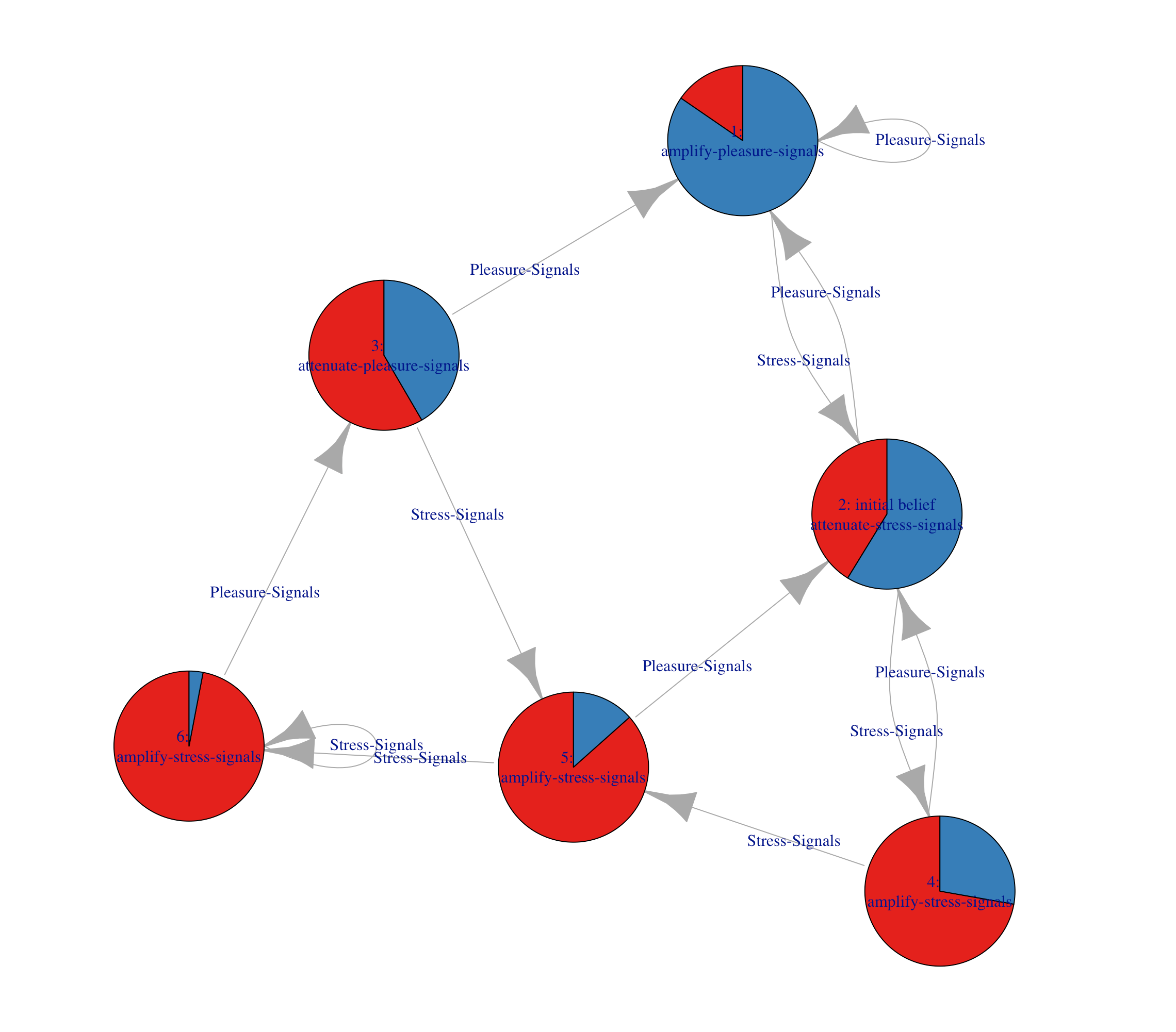
The optimal policy can be visualised as a policy graph, in which
each node corresponds to a conditional plan and edges represent
transitions triggered by observations. The graph is rendered using
plot_policy_graph():
plot_policy_graph(sol)
The value function $V^*(b)$ — piecewise linear and convex over the
belief simplex $\Delta(S)$ — is plotted as a function of the belief
coordinate $b(\texttt{Stressful}) \in [0, 1]$ using
plot_value_function():
plot_value_function(sol, ylim = c(-2, 1))
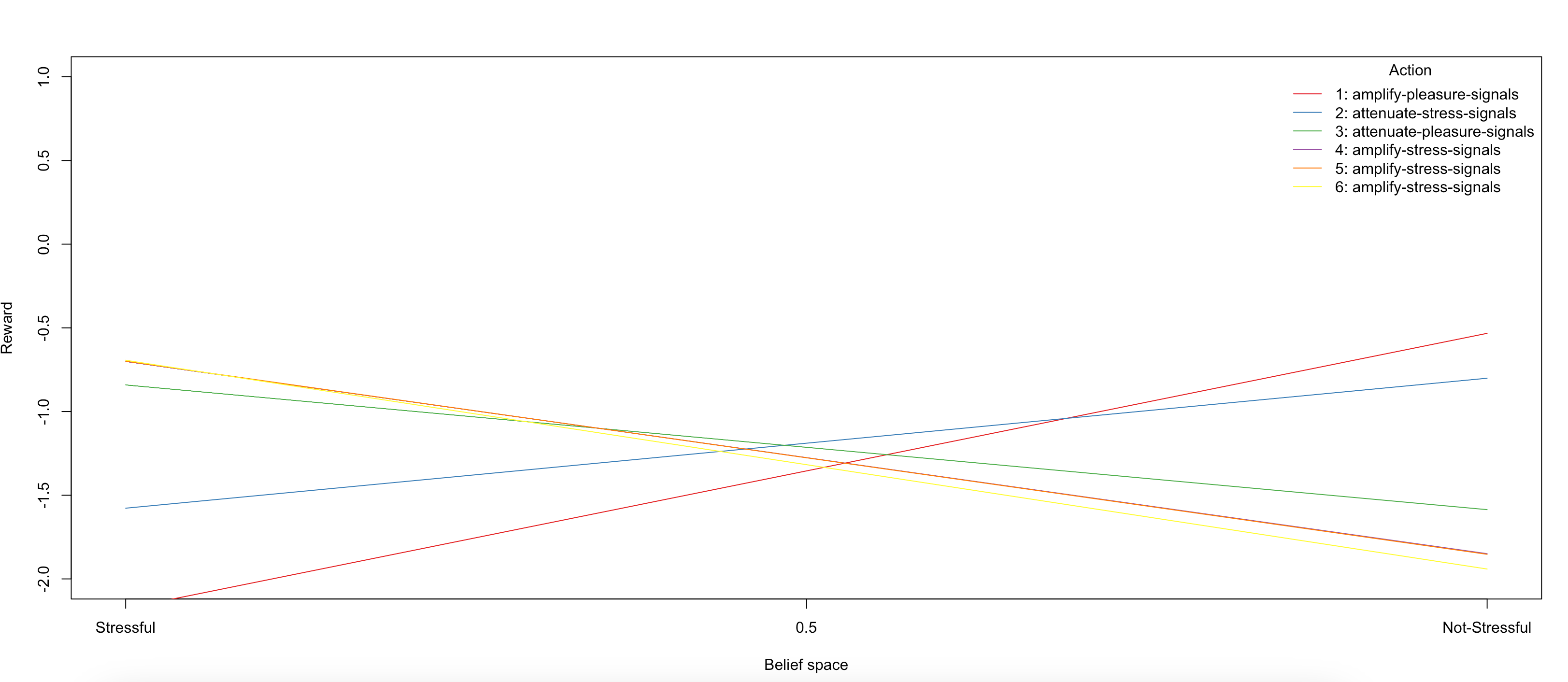
Each linear segment of the value function corresponds to a distinct $\alpha$-vector, representing the expected discounted return under a specific conditional plan. The convex envelope of these $\alpha$-vectors constitutes $V^(b)$, and the action associated with the dominating $\alpha$-vector at any belief point defines the optimal action $\pi^(b)$ at that point.
References
- POMDP package vignette — CRAN
- Partially Observable Markov Decision Processes — UBC CPSC 522
- Clark JE, Watson S. Modelling mood updating: a proof of principle study. Br J Psychiatry. 2023;222(3):125–134. doi:[10.1192/bjp.2022.175](doi:%5B10.1192/bjp.2022.175){.uri}. PMID: 36511113; PMCID: PMC9929713.
- Kurniawati H, Hsu D, Lee WS. SARSOP: Efficient point-based POMDP planning by approximating optimally reachable belief spaces. In: Proc. Robotics: Science and Systems. 2008.
- Littman ML, Cassandra AR, Kaelbling LP. Learning policies for partially observable environments: Scaling up. In: Proc. 12th International Conference on Machine Learning (ICML). San Francisco: Morgan Kaufmann; 1995. pp. 362–370.
- Pineau J, Gordon G, Thrun S. Point-based value iteration: An anytime algorithm for POMDPs. In: Proc. 18th International Joint Conference on Artificial Intelligence (IJCAI). San Francisco: Morgan Kaufmann; 2003. pp. 1025–1030.