Bayesian Gaussian Mixture Models
In statistics, a mixture model is a probabilistic model used to represent the presence of subpopulations within an overall population without requiring that an individual belongs to a specific subpopulation. It is a flexible approach that can be used to model complex data containing multiple regions with high probability mass, such as multimodal distributions. A typical finite-dimensional mixture model consists of observed random variables, random latent variables specifying the identity of the mixture component of each observation, mixture weights, and parameters. Mixture models can be used to make statistical inferences about the properties of subpopulations without sub-population identity information. Mixture models are also referred to as latent class models if they assume that some of their parameters differ across unobserved subgroups or classes.
Bayesian mixture models can be implemented in Stan, a probabilistic programming language. Mixture models assume that a given measurement can be drawn from one of K data generating processes, each with their own set of parameters. Stan allows for the fitting of Bayesian mixture models using its Hamiltonian Monte Carlo sampler. The models can be parameterized in several ways (see below) and used directly for modeling data with multimodal distributions or as priors for other parameters. The implementation of mixture models in Stan involves defining the model, specifying the priors, and marginalizing out the discrete parameters. Several resources provide examples and tutorials on fitting Bayesian mixture models in Stan, demonstrating the practical implementation of these models.
In this post I will first introduce how mixture models are implemented in Bayesian inference. It is noteworthy to take into consideration non-identifiability inherent these models how the non-identifiability can be tempered with principled prior information. Michael Betancourt has a blogpost describing the problems often encountered with gaussian mixture models, specifically the estimation of parameters of a mixture model and identifiability i.e. the problem with labelling mixtures.
Single varaible example
Data Simulation
library(dplyr)
library(ggplot2)
library(ggthemes)

N <- 500

#  three clusters
mu <- c(1, 4, 9)
sigma <- c(1.2, 1, 0.8)

# probability of each cluster
Theta <- c(.3, .5, .3)

# Draw which model each belongs to
z <- sample(1:3, size = N, prob = Theta, replace = T)

# white noise
epsilon <- rnorm(N)

# Simulate the data using the fact that y ~ normal(mu, sigma) can be
# expressed as y = mu + sigma*epsilon for epsilon ~ normal(0, 1)
y <- mu[z] + sigma[z]*epsilon

data_frame(y= y, z = as.factor(z)) %>%
  ggplot(aes(x = y, fill = z)) +
  geom_density(alpha = 0.3) +
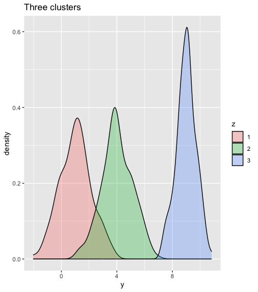
  ggtitle("Three clusters")

Stan model: code and description
mixture_model<-'

// saved as finite_mixture_linear_regression.stan
data {
  int N;
  vector[N] y;
  int n_groups;
}
parameters {
  vector[n_groups] mu;
  vector<lower = 0>[n_groups] sigma;
  simplex[n_groups] Theta;
}
model {
  vector[n_groups] contributions;
  // priors
  mu ~ normal(0, 10);
  sigma ~ cauchy(0, 2);
  Theta ~ dirichlet(rep_vector(2.0, n_groups));


  // likelihood
  for(i in 1:N) {
    for(k in 1:n_groups) {
      contributions[k] = log(Theta[k]) + normal_lpdf(y[i] | mu[k], sigma[k]);
    }
    target += log_sum_exp(contributions);
  }
}'
Data Block
N: Number of observations.y: Vector of observed responses.n_groups: Number of mixture components or groups.
Parameters Block
mu: Vector of means for each mixture component.sigma: Vector of standard deviations for each mixture component.Theta: Vector of mixing proportions, representing the probability of each group.
Model Block
- Priors: Normal priors are specified for the means
muwith a mean of 0 and a standard deviation of 10. Cauchy priors are specified for the standard deviationssigmawith a location of 0 and a scale of 2. Dirichlet priors are specified for the mixing proportionsThetawith equal concentration parameters of 2.0 for each group. - Likelihood: The likelihood is constructed within a nested loop. For each observation
iand each groupk, it calculates the log-likelihood of the observation given the mean and standard deviation of that group. These log-likelihoods are stored in thecontributionsvector. - Log-Sum-Exp Trick: To avoid numerical instability when dealing with small probabilities, the log-sum-exp trick is used. The
log_sum_expfunction sums up the contributions after exponentiating them. This is done to compute the log-likelihood of the data given the mixture model. - Target: The
targetis incremented by the log of the sum of exponentiated contributions for each observation. Thetargetis essentially the log-posterior, and the goal of Stan is to maximize it during sampling.
Fitting and output
library(rstan)
options(mc.cores = parallel::detectCores())

fit=stan(model_code=mixture_model, data=list(N= N, y = y, n_groups = 3), iter=3000, warmup=500, chains=3)


print(fit)
params=extract(fit)
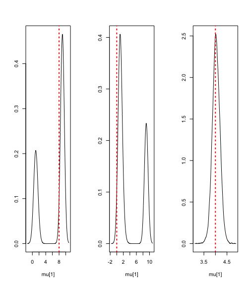
#density plots of the posteriors of the mixture means
par(mfrow=c(1,3))
plot(density(params$mu[,1]), ylab='', xlab='mu[1]', main='')
abline(v=c(8), lty='dotted', col='red',lwd=2)


plot(density(params$mu[,2]), ylab='', xlab='mu[1]', main='')
abline(v=c(0), lty='dotted', col='red',lwd=2)

plot(density(params$mu[,3]), ylab='', xlab='mu[1]', main='')
abline(v=c(4), lty='dotted', col='red',lwd=2)
Inference for Stan model: 9c40393d28e90e2c335fff95de690860.
3 chains, each with iter=3000; warmup=500; thin=1;
post-warmup draws per chain=2500, total post-warmup draws=7500.

             mean se_mean   sd     2.5%      25%      50%      75%    97.5% n_eff  Rhat
mu[1]        6.35    3.06 3.76     0.65     1.21     8.96     9.02     9.11     2 21.87
mu[2]        3.72    3.05 3.74     0.59     0.94     1.25     8.96     9.09     2 13.86
mu[3]        4.03    0.00 0.17     3.71     3.92     4.03     4.14     4.36  2575  1.00
sigma[1]     0.85    0.17 0.23     0.62     0.69     0.73     1.02     1.41     2  2.32
sigma[2]     1.01    0.19 0.27     0.64     0.73     1.03     1.19     1.60     2  1.76
sigma[3]     1.13    0.00 0.12     0.92     1.05     1.12     1.20     1.39  3232  1.00
Theta[1]     0.27    0.00 0.04     0.19     0.25     0.27     0.29     0.34  1186  1.02
Theta[2]     0.27    0.00 0.05     0.18     0.24     0.26     0.29     0.40  1553  1.00
Theta[3]     0.47    0.00 0.06     0.32     0.44     0.47     0.51     0.57  1702  1.00
lp__     -1161.00    0.05 2.18 -1166.34 -1162.15 -1160.64 -1159.40 -1157.91  2064  1.00

Samples were drawn using NUTS(diag_e) at Tue Feb  6 13:03:03 2024.
For each parameter, n_eff is a crude measure of effective sample size,
and Rhat is the potential scale reduction factor on split chains (at
convergence, Rhat=1).

Example with multiple variable
Data Simulation
library(MASS)

#first cluster
mu1=c(0,0,0,0)
sigma1=matrix(c(0.2,0,0,0,0,0.2,0,0,0,0,0.1,0,0,0,0,0.1),ncol=4,nrow=4, byrow=TRUE)
norm1=mvrnorm(30, mu1, sigma1)

#second cluster
mu2=c(10,10,10,10)
sigma2=sigma1
norm2=mvrnorm(30, mu2, sigma2)

#third cluster
mu3=c(4,4,4,4)
sigma3=sigma1
norm3=mvrnorm(30, mu3, sigma3)

norms=rbind(norm1,norm2,norm3) #combine the 3 mixtures together
N=90 #total number of data points
Dim=4 #number of dimensions
y=array(as.vector(norms), dim=c(N,Dim))
mixture_data=list(N=N, D=4, K=3, y=y)

as.data.frame(norms)  %>%
  pivot_longer(colnames(as.data.frame(norms)), names_to = "var", values_to = "value")%>%
  ggplot( aes(x=value, color=var)) + geom_density() +
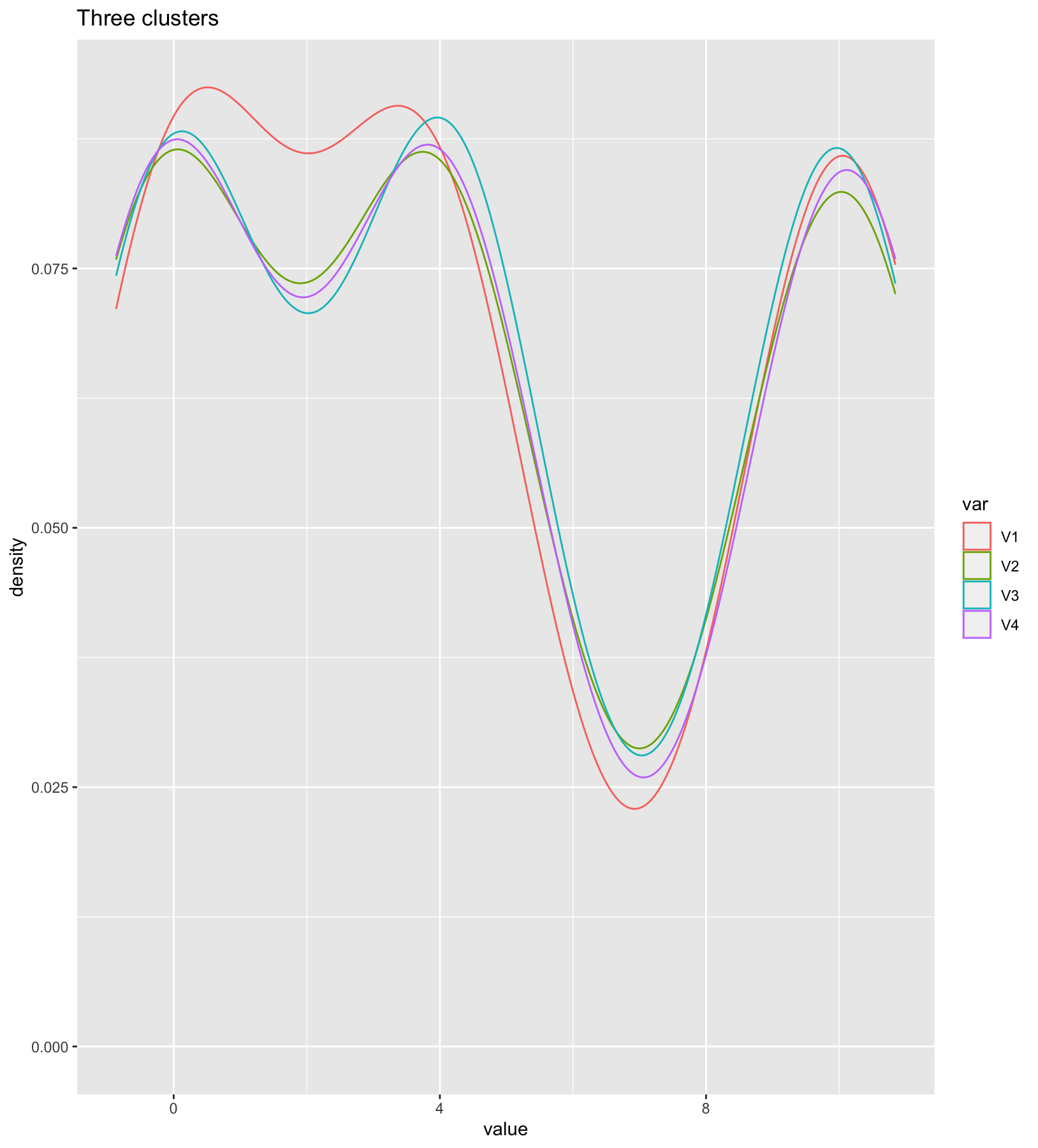
  ggtitle("Three clusters on four variables")

Stan model: code and description
mixture_model<-'
data {
 int D; //number of dimensions
 int K; //number of gaussians
 int N; //number of data
 vector[D] y[N]; //data
}

parameters {
 simplex[K] theta; //mixing proportions
 ordered[D] mu[K]; //mixture component means
 cholesky_factor_corr[D] L[K]; //cholesky factor of covariance
}

model {
 real ps[K];

 for(k in 1:K){
 mu[k] ~ normal(0,3);
 L[k] ~ lkj_corr_cholesky(4);
 }


 for (n in 1:N){
 for (k in 1:K){
 ps[k] = log(theta[k])+multi_normal_cholesky_lpdf(y[n] | mu[k], L[k]);
 }
 target += log_sum_exp(ps);
 }

}'
Data Block
D: Number of dimensions.K: Number of Gaussian components.N: Number of data points.y: An array of vectors, each representing a data point in D dimensions.
Parameters Block
theta: Mixing proportions. It is a simplex, ensuring that the proportions sum to 1.mu: Mixture component means. These are ordered variables.L: Cholesky factors of the covariance matrices for each component.
Model Block
-
Priors: Priors are specified for the means
muand the Cholesky factorsL. Each mean is drawn from a normal distribution with a mean of 0 and a standard deviation of 3. The Cholesky factor is drawn from a LKJ correlation distribution with shape parameter 4. -
Log-Probability Calculation: For each data point
nand each componentk, the log-probabilityps[k]is calculated. This log-probability is the logarithm of the product of the mixing proportion and the multivariate normal density of the data point under the k-th component. -
Target Increment: The
targetis incremented by the logarithm of the sum of exponentiated log-probabilitiesps. This step ensures that the model assigns higher probability to data points that are well-explained by one of the Gaussian components.
Fitting and output
fit=stan(model_code=mixture_model, data=mixture_data, iter=3000, warmup=1000, chains=1)
print(fit)

Inference for Stan model: f913dae683b9f29657b0863fec348d71.
1 chains, each with iter=3000; warmup=1000; thin=1;
post-warmup draws per chain=2000, total post-warmup draws=2000.

            mean se_mean   sd    2.5%     25%     50%     75%   97.5% n_eff Rhat
theta[1]    0.33    0.00 0.05    0.24    0.30    0.33    0.37    0.43  2120 1.00
theta[2]    0.33    0.00 0.05    0.24    0.30    0.33    0.36    0.44  1740 1.00
theta[3]    0.33    0.00 0.05    0.24    0.30    0.33    0.37    0.43  1854 1.00
mu[1,1]     3.80    0.00 0.11    3.55    3.74    3.80    3.86    3.99   632 1.01
mu[1,2]     3.91    0.01 0.12    3.67    3.84    3.90    3.98    4.15   236 1.00
mu[1,3]     4.02    0.01 0.13    3.78    3.92    4.02    4.11    4.29   344 1.00
mu[1,4]     4.09    0.01 0.15    3.82    3.99    4.09    4.20    4.39   259 1.00
mu[2,1]     9.77    0.01 0.12    9.51    9.70    9.79    9.86    9.98   405 1.00
mu[2,2]     9.96    0.00 0.11    9.74    9.90    9.96   10.03   10.20   794 1.00
mu[2,3]    10.09    0.00 0.11    9.91   10.01   10.07   10.15   10.33   518 1.00
mu[2,4]    10.18    0.01 0.12    9.97   10.09   10.17   10.25   10.43   498 1.00
mu[3,1]    -0.22    0.01 0.13   -0.49   -0.30   -0.21   -0.14    0.01   409 1.01
mu[3,2]    -0.10    0.01 0.13   -0.37   -0.17   -0.09   -0.02    0.17   218 1.00
mu[3,3]     0.07    0.01 0.13   -0.17    0.00    0.07    0.15    0.36    81 1.00
mu[3,4]     0.16    0.01 0.12   -0.03    0.08    0.15    0.23    0.42   541 1.00

For each parameter, n_eff is a crude measure of effective sample size,
and Rhat is the potential scale reduction factor on split chains (at
convergence, Rhat=1).
params=extract(fit)
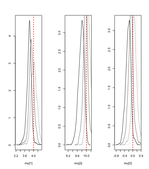
#density plots of the posteriors of the mixture means
par(mfrow=c(1,3))
plot(density(params$mu[,1,1]), ylab='', xlab='mu[1]', main='')
lines(density(params$mu[,1,2]), col=rgb(0,0,0,0.7))
lines(density(params$mu[,1,3]), col=rgb(0,0,0,0.4))
lines(density(params$mu[,1,4]), col=rgb(0,0,0,0.1))
abline(v=c(4), lty='dotted', col='red',lwd=2)

plot(density(params$mu[,2,1]), ylab='', xlab='mu[2]', main='')
lines(density(params$mu[,2,2]), col=rgb(0,0,0,0.7))
lines(density(params$mu[,2,3]), col=rgb(0,0,0,0.4))
lines(density(params$mu[,2,4]), col=rgb(0,0,0,0.1))
abline(v=c(10), lty='dotted', col='red',lwd=2)

plot(density(params$mu[,3,1]), ylab='', xlab='mu[3]', main='')
lines(density(params$mu[,3,2]), col=rgb(0,0,0,0.7))
lines(density(params$mu[,3,3]), col=rgb(0,0,0,0.4))
lines(density(params$mu[,3,4]), col=rgb(0,0,0,0.1))
abline(v=c(0), lty='dotted', col='red',lwd=2)

Advantages and Limitations
Bayesian mixture models offer several advantages in statistical modeling. Their inherent flexibility makes them well-suited for diverse tasks such as clustering, data compression, outlier detection, and generative classification. The Bayesian framework’s ability to incorporate prior knowledge enhances model accuracy, especially when informative prior information is available. Moreover, these models effectively handle unobserved heterogeneity by integrating multiple data generating processes, proving valuable when data alone may not fully identify underlying patterns. The stability provided by Bayesian estimation ensures reliable posterior distributions, reducing sensitivity to issues like singularities, over-fitting, and violated identification criteria. Bayesian mixture models also facilitate the examination of the posterior distribution of the number of classes, offering insights into the underlying class structure of the data. However, the use of Bayesian mixture models comes with certain limitations. Applying these models demands a high level of statistical expertise to appropriately specify priors and ensure correct model formulation, presenting a challenge for practitioners lacking a strong background in Bayesian statistics. The complexity of posterior inference is compounded by label switching, a phenomenon that complicates the interpretation of results. Bayesian nonparametric mixture models, in particular, may suffer from inconsistency in estimating the number of clusters, impacting their performance in clustering applications. Additionally, model fitting challenges arise, and careful evaluation of inaccuracies in predictions and comparison with alternative models are essential to address potential shortcomings.
In this post, we learned to fit mixture models using Stan. We saw how to evaluate model fit using the usual prior and posterior predictive checks, and to investigate parameter recovery. Such mixture models are notoriously difficult to fit, but they have a lot of potential in cognitive science applications, especially in developing computational models of different kinds of cognitive processes. The reader interested in a deeper understanding of potential challanges in the process can refer to Betancourt discussion of identification problems in Bayesian mixture models in a case study.
References
- Finite mixture models in Stan
- Multivariate Gaussian Mixture Model done properly
- Finite Mixtures
- Identifying Bayesian Mixture Models
- Mixture models
- Bayesian Density Estimation (Finite Mixture Model)
- Bayesian mixture models (in)consistency for the number of clusters
- Advantages of a Bayesian Approach for Examining Class Structure in Finite Mixture Models
