Dirichlet Regression and Clustering in R
The Dirichlet distribution can be used in both regression and clustering models when analyzing proportional data, data that represents proportions summing to 1, such as percentages. In the R programming language, two powerful packages, DirichletReg for regression and dirichletprocess for clustering, offer versatile tools for analyzing such data through Bayesian approaches.
Dirichlet Regression with the DirichletReg Package
Dirichlet regression provides a robust framework for modeling compositional data frequently found in fields like ecology, economics, and social sciences. The DirichletReg package in R is specifically designed to perform regression analysis where the response variables are proportions. It allows for the estimation of the relationship between these proportions and various predictors, making it an essential tool for research involving data that reflects parts of a whole. The package offers two key parametrizations for model specification: one using α (common parametrization) and another using μ/φ (alternative parametrization), providing flexibility in model interpretation. The package also includes a variety of diagnostic and visualization tools, such as residual plots and confidence intervals, allowing for a more comprehensive evaluation of model performance. To use the package, the dependent variable, which consists of compositional data, needs to be converted into a special format using the DR_data() function. This function ensures that the data is properly structured for Dirichlet regression analysis. The main function for fitting Dirichlet regression models is DirichReg(). It allows users to specify the model formula, choose the parametrization, and include various predictors. The formula syntax is similar to other regression functions in R, making it intuitive for users familiar with R’s modeling framework. Once a model is fitted, the package provides several methods for analyzing and interpreting the results. These include summary() for model summaries, predict() for generating predictions, and various diagnostic tools such as residual plots and confidence intervals. The package also includes functions for model comparison, such as anova(), which enables researchers to compare nested models and assess the significance of additional predictors or more complex model structures. Likewise, the package provides plotting functions that allow users to create informative visualizations of their compositional data and model results.
Dirichlet Process Clustering with the dirichletprocess Package
Dirichlet process clustering focuses on unsupervised learning, offering a nonparametric Bayesian approach that automatically determines the number of clusters in the data. The dirichletprocess package in R implements Dirichlet process mixture models (DPMMs), which are particularly useful when the number of clusters is unknown or difficult to pre-specify. This method is useful for exploratory data analysis, as it takes into consideration to the underlying structure of the data, making it highly flexible. The dirichletprocess package simplifies the implementation of Dirichlet process clustering by providing functions for creating mixture models using a variety of distributions, including Normal, Multivariate Normal, Beta, and Weibull distributions. These models can then be fitted using Markov Chain Monte Carlo (MCMC) methods to estimate cluster memberships. The package automatically handles complex tasks like tuning hyperparameters and selecting the number of clusters based on the data, relieving the user from manually specifying these parameters. The key advantage of Dirichlet processes is that they do not require specifying the number of clusters beforehand. Instead, the model adapts to the data, automatically determining the number of clusters based on the observed patterns. To run a clustering model with the ‘dirichletprocess’ package the data should be scaled or normalized as appropriate for the chosen kernel distribution. For instance, the Multivariate Normal Kernel (MNK) is often used for continuous multivariate data followed by the MCMC sampling algorithm, which estimates the posterior distribution of the model parameters. Finally after fitting, the package provides methods to extract cluster assignments and visualize the results.
Both the DirichletReg and dirichletprocess packages highlight the usefulness and flexibility of the Dirichlet distribution in handling a variety of data structures, from compositional/proportional to clustered. These tools allow researchers to approach their analyses in a Bayesian framework, providing more natural inferences about uncertainty and the data-generating process. As such, they have become essential in domains where proportions and clustering play central roles.
Dirichlet Regression Example
First, we load the DirichletReg package and the built-in ArcticLake dataset.
# Load the DirichletReg package
library(DirichletReg)

# Load the ArcticLake dataset
data(ArcticLake)

# View the first few rows of the dataset
head(ArcticLake)
We use the DR_data() function to prepare the data for Dirichlet regression. This function processes the first three columns of ArcticLake (representing proportions of sand, silt, and clay) and ensures that each row sums to 1, a requirement for compositional data.
# Prepare the data for Dirichlet regression
AL <- DR_data(ArcticLake[, 1:3])
Using the DirichReg() function, we fit a Dirichlet regression model. In the formula AL ~ depth, depth is specified as the predictor for the compositional outcome AL (sand, silt, and clay proportions).
# Fit a Dirichlet regression model
model <- DirichReg(AL ~ depth, ArcticLake)
The summary() function provides a detailed overview of the fitted model, including coefficient estimates, significance levels, and diagnostics.
# Display the model summary
summary(model)

DirichReg(formula = AL ~ depth, data = ArcticLake)

Standardized Residuals:
          Min       1Q   Median      3Q     Max
sand  -1.7724  -0.8319   0.0120  1.3435  2.2862
silt  -1.0863  -0.5343  -0.1279  0.2892  1.4493
clay  -2.0868  -0.7516  -0.0012  0.4391  1.9660

------------------------------------------------------------------
Beta-Coefficients for variable no. 1: sand
            Estimate Std. Error z value Pr(>|z|)
(Intercept) 0.116625   0.409292   0.285  0.77569
depth       0.023351   0.007454   3.133  0.00173 **
------------------------------------------------------------------
Beta-Coefficients for variable no. 2: silt
             Estimate Std. Error z value Pr(>|z|)
(Intercept) -0.310596   0.344731  -0.901    0.368
depth        0.055567   0.006365   8.730   <2e-16 ***
------------------------------------------------------------------
Beta-Coefficients for variable no. 3: clay
             Estimate Std. Error z value Pr(>|z|)
(Intercept) -1.151956   0.298473   -3.86 0.000114 ***
depth        0.064302   0.005738   11.21  < 2e-16 ***
------------------------------------------------------------------
Significance codes: 0 ‘***’ 0.001 ‘**’ 0.01 ‘*’ 0.05 ‘.’ 0.1 ‘ ’ 1

Log-likelihood: 101.4 on 6 df (98 BFGS + 1 NR Iterations)
AIC: -190.7, BIC: -180.8
Number of Observations: 39
Link: Log
Parametrization: common
To make predictions across a range of depth values, we create a new dataset (new_data) with a sequence of depth values spanning the full range of depths in the original data.
# Create a sequence of depth values for predictions
new_data <- data.frame(depth = seq(min(ArcticLake$depth), max(ArcticLake$depth), length.out = 100))
head(new_data)
Using the predict() function, we generate predictions from the model for the new depth values, allowing us to examine how the composition changes with depth.
# Make predictions based on the fitted model
predictions <- predict(model, new_data)
head(predictions)
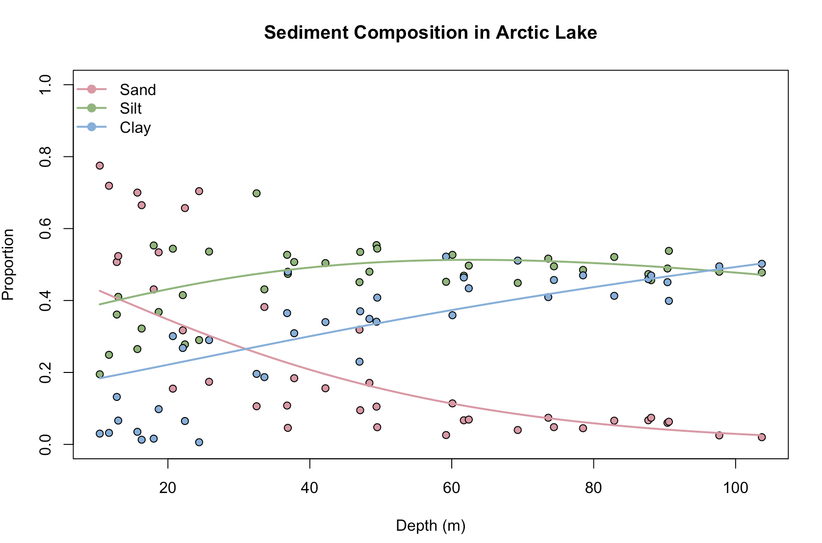
we also can visualize the results:
# Plot the original data points and predictions
plot(rep(ArcticLake$depth, 3), as.numeric(AL), pch = 21,
     bg = rep(c("#E495A5", "#86B875", "#7DB0DD"), each = nrow(ArcticLake)),
     xlab = "Depth (m)", ylab = "Proportion", ylim = 0:1,
     main = "Sediment Composition in Arctic Lake")

# Add lines for each component prediction
for (i in 1:3) {
  lines(new_data$depth, predictions[, i], col = c("#E495A5", "#86B875", "#7DB0DD")[i], lwd = 2)
}

# Add a legend
legend("topleft", legend = c("Sand", "Silt", "Clay"), lwd = 2,
       col = c("#E495A5", "#86B875", "#7DB0DD"), pt.bg = c("#E495A5", "#86B875", "#7DB0DD"),
       pch = 21, bty = "n")

Dirichlet clustering Example
This example demonstrates how to perform Dirichlet process clustering on the faithful dataset, which contains two variables: eruption duration and waiting time for Old Faithful geyser eruptions. Here’s a breakdown of each step in the text-code-text-code format to help you understand the process.
The faithful dataset is built into R, so we start by loading it and viewing the first few rows.
data("faithful")
head(faithful)
Since we’re clustering with a multivariate approach, we scale the data to standardize the eruption and waiting times.
faithfulTrans <- scale(faithful)
We ‘fit’ a Dirichlet Process Mixture Model with a multivariate normal kernel, well-suited for clustering continuous data. The Dirichlet process groups similar observations based on probabilistic clustering without requiring a fixed number of clusters.
dp <- DirichletProcessMvnormal(faithfulTrans)
# Fit the model using MCMC sampling for 1000 iterations
dp <- Fit(dp, 1000)
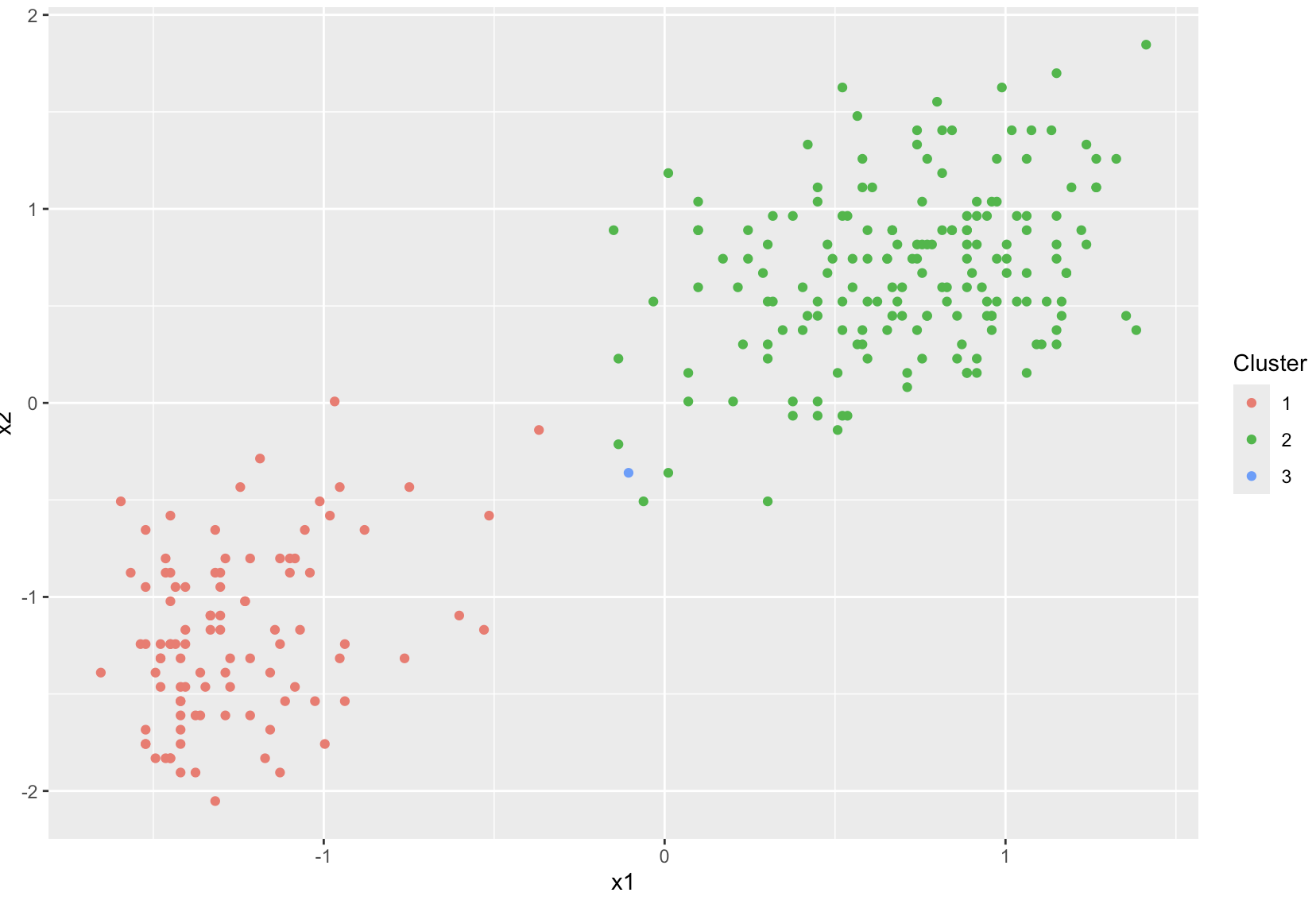
After fitting, we can plot the clusters. Each color in the plot represents a different cluster assignment.
# Plot the data points, colored by their cluster assignments
plot(dp)

You can obtain the clusterLabels for each data point to see which observations belong to which clusters.
# Get the cluster assignments
clusters <- dp$clusterLabels

# Display the cluster assignments
print(clusters)
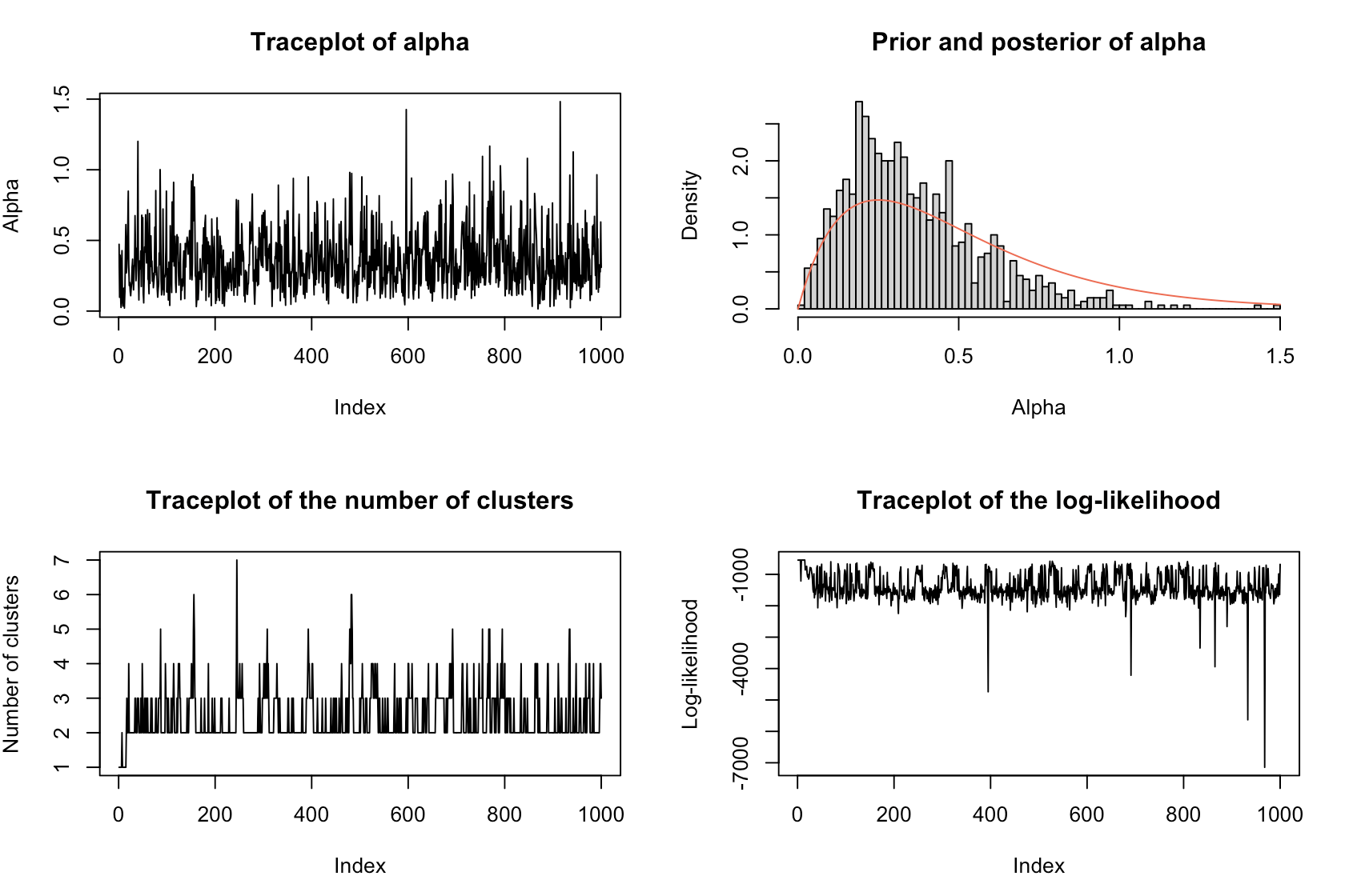
Diagnostic plot() of the Dirichlet process model provides details on the clustering results, while the posterior distribution shows the size of each cluster.
DiagnosticPlots(dp, gg = FALSE)

# Posterior distribution of cluster sizes
posterior_sizes <- table(clusters)
print(posterior_sizes)

Conclusion
The Dirichlet distribution is a useful tool for both regression and clustering applications. The DirichletReg package in R offers a robust framework for Dirichlet regression, which is ideal for modeling proportional data—data where the sum of components is constrained to 1. By providing flexible parametrizations (using α or μ/φ), diagnostic tools, and functions for model comparison and visualization, the package simplifies the process of drawing meaningful inferences about relationships in compositional data. Likewise, the Dirichletprocess package supports unsupervised learning through Dirichlet Process Mixture Models, a nonparametric Bayesian approach. This technique is especially useful when the number of clusters in a dataset is unknown or difficult to specify. Its flexibility, which allows the model to adapt based on data patterns, is useful for exploratory data analysis in domains such as bioinformatics. The package automates many of the challenging aspects of Bayesian inference, such as hyperparameter tuning and MCMC sampling, providing researchers with a user-friendly tool to uncover hidden structures in data. While these tools offer powerful capabilities, several questions remain for further exploration. How can Dirichlet regression models be further adapted to handle missing data or hierarchical structures in datasets? Can interaction terms or more complex non-linear relationships be better accommodated in the current framework? In what ways can we improve the interpretability of Dirichlet regression coefficients, particularly when dealing with complex, multi-component responses? How does Dirichlet process clustering perform when applied to extremely high-dimensional data, such as in genomics or image recognition? What strategies can enhance the scalability of Dirichlet process models for larger datasets? Exploring these questions could lead to new applications for the Dirichlet distribution in both supervised and unsupervised learning contexts.
References
- Package DirichletReg: Regression Analysis with Dirichlet Distributions
- Dirichlet Regression With R
- DirichletReg Vignette
- Austrian Research Report - Dirichlet Analysis
- CRAN R Package: DirichletReg
- Data Science Tutorials: Clustering
- R Documentation: Dirichlet Process
- Dirichlet Process: A CRAN Vignette
- OhioLink Thesis - Dirichlet Regression
- Iieta Research Report - Dirichlet Processes
- Dirichlet Regression Discussion on Stan Forum
- R Package DirReg - Beta Discussion on Stan Forum
- ZOID R Package Documentation
- ArXiv Preprint: Dirichlet Regression Models
- GitHub: Dirichlet Process
- Dirichlet Process CRAN Documentation
