Chapter 11 Bayesian Seasonal Decomposition in Stan and RStan
Understanding the components that make up a time series is a critical first step in analysis and forecasting. Classical seasonal decomposition techniques, such as STL or X-11, offer ways to separate a series into trend, seasonal, and irregular components. However, these methods are often deterministic and lack a coherent probabilistic framework for uncertainty quantification.
In contrast, Bayesian seasonal decomposition allows us to model uncertainty in each component explicitly. In this post, we demonstrate how to construct a Bayesian structural time series model in Stan, decompose a seasonal time series, and obtain posterior distributions for each latent component.
11.1 Simulating Seasonal Time Series Data*
We first simulate a synthetic time series with additive trend, seasonality, and noise:
set.seed(123)
n <- 120
t <- 1:n
trend <- 0.05 * t
seasonal_period <- 12
seasonal <- rep(sin(2 * pi * (1:seasonal_period) / seasonal_period), length.out = n)
noise <- rnorm(n, 0, 0.5)
y <- trend + seasonal + noise

ts.plot(y, main = "Simulated Time Series with Trend and Seasonality")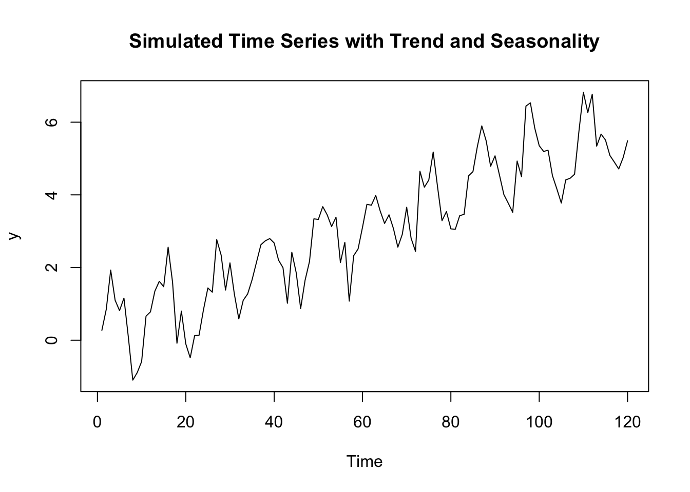
11.2 Bayesian Seasonal Decomposition Model in Stan
We use an additive structural model:
\[ y_t = \mu_t + \gamma_t + \epsilon_t \]
- \(\mu_t\): Local level (trend)
- \(\gamma_t\): Seasonal component
- \(\epsilon_t \sim \mathcal{N}(0, \sigma^2)\): Irregular component
We impose a local level model for the trend:
\[ \mu_t = \mu_{t-1} + \eta_t, \quad \eta_t \sim \mathcal{N}(0, \sigma_{\mu}^2) \]
And we model seasonality with a constraint that its sum over one period equals zero (to ensure identifiability):
stan_model_1 <-'data {
  int<lower=2> N;
  int<lower=2> s;           // seasonal period
  vector[N] y;
}
parameters {
  vector[N] mu;             // trend
  vector[s] season_raw;     // raw seasonal effects
  real<lower=0> sigma;
  real<lower=0> sigma_mu;
  real<lower=0> sigma_season;
}
transformed parameters {
  vector[N] season;
  vector[s] season_clean;

  // Center seasonal component to sum to zero
  season_clean = season_raw - mean(season_raw);

  for (t in 1:N)
    season[t] = season_clean[1 + ((t - 1) % s)];
}
model {
  mu[2:N] ~ normal(mu[1:(N - 1)], sigma_mu);
  season_raw ~ normal(0, sigma_season);
  y ~ normal(mu + season, sigma);
}'
11.3 Fitting the Model in R
We fit this model using RStan:
library(rstan)

data_list <- list(
  N = length(y),
  s = seasonal_period,
  y = y
)

fit <- stan(
  model_code = stan_model_1,
  data = data_list,
  chains = 4,
  iter = 2000,
  warmup = 1000,
  seed = 123
)
## Warning: Bulk Effective Samples Size (ESS) is too low, indicating posterior means and medians may be unreliable.
## Running the chains for more iterations may help. See
## https://mc-stan.org/misc/warnings.html#bulk-ess## Inference for Stan model: anon_model.
## 4 chains, each with iter=2000; warmup=1000; thin=1;
## post-warmup draws per chain=1000, total post-warmup draws=4000.
##
## mean se_mean sd 2.5% 25% 50% 75% 97.5% n_eff Rhat
## sigma 0.42 0 0.04 0.36 0.40 0.42 0.44 0.50 3026 1.00
## sigma_mu 0.18 0 0.04 0.13 0.16 0.18 0.20 0.26 319 1.01
## sigma_season 0.81 0 0.22 0.50 0.66 0.77 0.91 1.33 2846 1.00
##
## Samples were drawn using NUTS(diag_e) at Wed Oct 1 09:45:01 2025.
## For each parameter, n_eff is a crude measure of effective sample size,
## and Rhat is the potential scale reduction factor on split chains (at
## convergence, Rhat=1).11.4 Extracting and Visualizing Components
We now extract the posterior estimates and visualize the trend and seasonal components:
posterior <- extract(fit)
mu_hat <- apply(posterior$mu, 2, mean)
season_hat <- apply(posterior$season, 2, mean)

par(mfrow = c(3, 1), mar = c(4, 4, 2, 1))
plot(y, type = 'l', main = "Observed Time Series", ylab = "y")
plot(mu_hat, type = 'l', col = "blue", main = "Estimated Trend (mu)", ylab = "mu_t")
plot(season_hat, type = 'l', col = "darkgreen", main = "Estimated Seasonal Component", ylab = "season_t")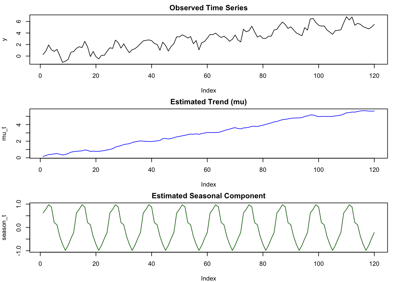
This visual decomposition gives insight into how much of the variation is driven by the underlying trend and how much by recurring seasonal patterns. The Bayesian framework also allows for full posterior uncertainty quantification, which can be visualized with credible intervals around each component.
11.5 Extensions and Applications
Bayesian structural time series models can be extended in numerous ways. One may introduce regression components to account for covariates (leading to models like BSTS), or allow the trend to include a slope (i.e., a local linear trend). Multivariate or hierarchical seasonal decomposition is also possible and particularly useful for grouped or panel time series.
11.6 Conclusion
Bayesian seasonal decomposition offers a principled approach to breaking down time series into interpretable components while rigorously accounting for uncertainty. Compared to classical methods, the Bayesian formulation in Stan provides flexibility, interpretability, and extensibility. Whether used for exploratory analysis or as a preprocessing step for forecasting, structural time series decomposition is a valuable tool in the Bayesian modeler’s toolkit.