Stock Forecasting with LSTM
Introduction
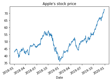
As indicated in a previous blog post, time-series models are designed to predict future values based on previously observed values. In other words the input is a signal (time-series) that is defined by observations taken sequentially in time. However, time-series forecasting models such as ARIMA has it own limitations when it comes to non-stationary data (i.e. where statistical properties e.g. the mean and standard deviation are not constant over time but instead, these metrics vary over time). An examples of non-stationary time-series stock price (not to be confused with stock returns) over time.
As discussed in a previous blog post here there have been attempts to predict stock outcomes (e.g. price, return. etc.) using time series analysis algorithms, though the performance is sub par and cannot be used to efficiently predict the market. It is noteworthy that this is a technical tutorial and does not intent to guide people into buying stocks.
LSTM
The LSTM stands for Long Short-Term Memory a member of recurrent neural network (RNN) family used for sequence data in deep learning. Unlike standard feedforward fully connected neural network layers, RNNs and here LSTM have feedback loops which enables them to store information over a period of time also reffered to as a memory capacity.
import pandas as pd
import numpy as np
import matplotlib.pyplot as plt
import pandas as pd
from sklearn.preprocessing import MinMaxScaler
import yfinance as yf
from yahoofinancials import YahooFinancials
%matplotlib inline
The first step is to download the data from Yahoo finance. In the first step we focus on the Apple stock.
appl_df = yf.download('AAPL',
                      start='2018-01-01',
                      end='2019-12-31',
                      progress=False)
appl_df.head()
| Open | High | Low | Close | Adj Close | Volume | |
|---|---|---|---|---|---|---|
| Date | ||||||
| 2018-01-02 | 42.540001 | 43.075001 | 42.314999 | 43.064999 | 41.380238 | 102223600 |
| 2018-01-03 | 43.132500 | 43.637501 | 42.990002 | 43.057499 | 41.373032 | 118071600 |
| 2018-01-04 | 43.134998 | 43.367500 | 43.020000 | 43.257500 | 41.565216 | 89738400 |
| 2018-01-05 | 43.360001 | 43.842499 | 43.262501 | 43.750000 | 42.038452 | 94640000 |
| 2018-01-08 | 43.587502 | 43.902500 | 43.482498 | 43.587502 | 41.882305 | 82271200 |
and to plot it using pandas plotting function.
appl_df['Open'].plot(title="Apple's stock price")
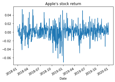
here we covert the stock price to daily stock returns and to plot it
appl_df['Open']=appl_df['Open'].pct_change()
appl_df['Open'].plot(title="Apple's stock return")
From previous experience with deep learning models, we know that we have to scale our data for optimal performance. In our case, we’ll use Scikit- Learn’s StandardScaler and scale our dataset to numbers between zero and one.
sc = StandardScaler()
here we create a univariate pre-processor function that does three steps of min max scaling, creating lags, and separating the data to train and test sets for a given time-series.
def preproc( data, lag, ratio):
    data=data.dropna().iloc[:, 0:1]
    Dates=data.index.unique()
    data.iloc[:, 0] = sc.fit_transform(data.iloc[:, 0].values.reshape(-1, 1))
    for s in range(1, lag):
        data['shift_{}'.format(s)] = data.iloc[:, 0].shift(s)
    X_data = data.dropna().drop(['Open'], axis=1)
    y_data = data.dropna()[['Open']]
    index=int(round(len(X_data)*ratio))
    X_data_train=X_data.iloc[:index,:]
    X_data_test =X_data.iloc[index+1:,:]
    y_data_train=y_data.iloc[:index,:]
    y_data_test =y_data.iloc[index+1:,:]
    return X_data_train,X_data_test,y_data_train,y_data_test,Dates;
Then we apply the univariate pre-processing to the Apple data
a,b,c,d,e=preproc(appl_df, 25, 0.90)
As a second ticker and an additional varaible to improve our model performance we focus of the SP500 index eft SPY.
spy_df = yf.download('SPY',
                      start='2018-01-01',
                      end='2019-12-31',
                      progress=False)
spy_df.head()
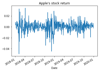
here we covert the stock price to daily stock returns and to plot it
spy_df['Open']=spy_df['Open'].pct_change()
spy_df['Open'].plot(title="Apple's stock return")
here we create a multi-variate pre-processor function that does three steps of min max scaling, creating lags, and separating the data to train and test sets for common dates of two time series.
def preproc2( data1, data2, lag, ratio):
    common_dates=list(set(data1.index) & set(data2.index))
    data1=data1[data1.index.isin(common_dates)]
    data2=data2[data2.index.isin(common_dates)]
    X1=preproc(data1, lag, ratio)
    X2=preproc(data2, lag, ratio)
    return X1,X2;
Then we apply the multi-variate pre-processing to both SPY and Apple data
dataLSTM=preproc2( spy_df, appl_df, 25, 0.90)
here we load necessary libraries for the deep learning model
from keras.models import Sequential
from keras.layers import Dense
from keras.layers import LSTM
import keras.backend as K
from keras.callbacks import EarlyStopping
in order to run the models data should be transformed to numpy arrays
a = a.values
b= b.values

c = c.values
d = d.values
and properly reshaped for LSTM modeling
X_train_t = a.reshape(a.shape[0], 1, 24)
X_test_t = b.reshape(b.shape[0], 1, 24)
here we define a simple Sequential model with two LSTM and two dense layers
K.clear_session()
early_stop = EarlyStopping(monitor='loss', patience=1, verbose=1)
model = Sequential()
model.add(LSTM(12, input_shape=(1, 24), return_sequences=True))
model.add(LSTM(6))
model.add(Dense(6))
model.add(Dense(1))
model.compile(loss='mean_squared_error', optimizer='adam')
that we train for 100 epochs
model.fit(X_train_t, c,
          epochs=100, batch_size=1, verbose=1,
          callbacks=[early_stop])


    Epoch 1/100
    429/429 [==============================] - 2s 1ms/step - loss: 1.3043
    Epoch 2/100
    429/429 [==============================] - 0s 1ms/step - loss: 0.9467
    ...
    Epoch 00029: early stopping
Here we create a rolling forecast function that predicts the values based on the previous outcomes of the model.
ypredr=[]
st=X_test_t[0].reshape(1, 1, 24)
tmp=st
ptmp=st
val=model.predict(st)
ypredr.append(val.tolist()[0])
for i in range(1, X_test_t.shape[0]):
    tmp=np.append(val, tmp[0,0, 0:-1])
    tmp=tmp.reshape(1, 1, 24)
    ptmp=np.vstack((ptmp,tmp))
    val=model.predict(tmp)
    ypredr.append(val.tolist()[0])
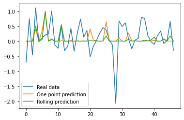
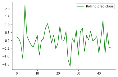
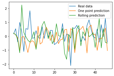
the plot here shows the rolling forecast which base each forecast on 24 data points forecasted beforehand, this should be contrasted to the one point forecast function that base each forecast on 24 data points observed beforehand.
plt.plot(ypredr,color="green", label = "Rolling prediction")
plt.legend()
plt.show()
y_pred = model.predict(X_test_t)
plt.plot(d, label = "Real data")
plt.plot(y_pred, label = "One point prediction")
plt.plot(ypredr, label = "Rolling prediction")
plt.legend()
plt.show()
 here we move to multivariate models. First, to run the models data should be transformed to numpy arrays.
Aa = dataLSTM[0][0].values
Ab = dataLSTM[0][1].values

Ac = dataLSTM[0][2].values
Ad = dataLSTM[0][3].values
X_train_A = Aa.reshape(Aa.shape[0], 1, 24)
X_test_A = Ab.reshape(Ab.shape[0], 1, 24)

Sa = dataLSTM[1][0].values
Sb = dataLSTM[1][1].values

Sc = dataLSTM[1][2].values
Sd = dataLSTM[1][3].values
X_train_S = Sa.reshape(Sa.shape[0], 1, 24)
X_test_S = Sb.reshape(Sb.shape[0], 1, 24)
here we load necessary libraries for the deep learning model
from keras.layers import concatenate
from keras.layers import Dropout
from keras.layers import Dense
import keras.backend as K
from keras.callbacks import EarlyStopping
from keras.layers import LSTM
from keras.models import Input, Model
from keras.layers import Dense
here we define model with Keras functional API using two LSTM layers concatenated together and two dense layers with drop out.
early_stop = EarlyStopping(monitor='loss', patience=1, verbose=1)
input1 = Input(shape=(1,24)) # for the three columns of dat_train
x1 = LSTM(6)(input1)

input2 = Input(shape=(1,24))
x2 = LSTM(6)(input2)

con = concatenate(inputs = [x1,x2] ) # merge in metadata
x3 = Dense(50)(con)
x3 = Dropout(0.3)(x3)
output = Dense(1, activation='sigmoid')(x3)
n_net = Model(inputs=[input1, input2], outputs=output)
n_net.compile(loss='mean_squared_error', optimizer='adam')
and to train the model for 100 epochs
n_net.fit(x=[X_train_A, X_train_S], y=Ac, epochs=100, batch_size=1, verbose=1,
          callbacks=[early_stop])


    Epoch 1/100
    429/429 [==============================] - 0s 832us/step - loss: 0.7942
    Epoch 2/100
    429/429 [==============================] - 0s 808us/step - loss: 0.7825
    ...
    Epoch 14/100
    429/429 [==============================] - 0s 802us/step - loss: 0.7143
    Epoch 00014: early stopping

    ```


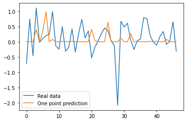
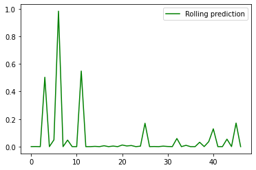
the plot here shows the rolling forecast which base each forecast on 24
data points forecasted beforehand, this should be contrasted to the one
point forecast function that base each forecast on 24 data points
observed beforehand.


``` {.python}
y_pred = n_net.predict([X_test_A,X_test_S])
plt.plot(Ad, label = "Real data")
plt.plot(y_pred, label = "One point prediction")
plt.legend()
plt.show()
ypredr=[]
st=X_test_A[0].reshape(1, 1, 24)
sst=X_test_S[0].reshape(1, 1, 24)
tmp=st
ptmp=st
val=n_net.predict([tmp,sst])
ypredr.append(val.tolist()[0])
for i in range(1, X_test_t.shape[0]):
    tmp=np.append(val, tmp[0,0, 0:-1])
    tmp=tmp.reshape(1, 1, 24)
    sst=X_test_S[i].reshape(1, 1, 24)
    ptmp=np.vstack((ptmp,tmp))
    val=n_net.predict([tmp,sst])
    ypredr.append(val.tolist()[0])
plt.plot(ypredr, color="green", label = "Rolling prediction")
plt.legend()
plt.show()
y_pred = n_net.predict([X_test_A,X_test_S])
plt.plot(Ad, label = "Real data")
plt.plot(y_pred, label = "One point prediction")
plt.plot(ypredr, label = "Rolling prediction")
plt.legend()
plt.show()
