Introduction
As discussed in a previous blog post here there have been attempts to predict stock outcomes (e.g. price, return, etc.) using recurrent neural networks and more specifically LSTMs. The LSTM stands for Long Short-Term Memory a member of recurrent neural network (RNN) family used for sequence data in deep learning. Unlike standard feedforward fully connected neural network layers, RNNs and here LSTM have feedback loops which enables them to store information over a period of time also referred to as a memory capacity. The example above showed that the performance is sub par and cannot be used to efficiently predict the market. One approach is to tune hyperparameters of the network such as the number of layers, activation functions, and regularization. This tutorial aims to highlight the use of the Keras Tuner package to tune a LSTM network for time series analysis. It is noteworthy that this is a technical tutorial and does not intent to guide people into buying stocks.
import pandas as pd
import numpy as np
import matplotlib.pyplot as plt
import pandas as pd
from sklearn.preprocessing import StandardScaler
import yfinance as yf
from yahoofinancials import YahooFinancials
%matplotlib inline
The first step is to download the data from Yahoo finance. In the first step we focus on the Apple stock.
appl_df = yf.download('AAPL',
                      start='2019-01-01',
                      end='2020-12-31',
                      progress=False)

appl_df.head()
| Open | High | Low | Close | Adj Close | Volume | |
|---|---|---|---|---|---|---|
| Date | ||||||
| 2018-01-02 | 42.540001 | 43.075001 | 42.314999 | 43.064999 | 41.380238 | 102223600 |
| 2018-01-03 | 43.132500 | 43.637501 | 42.990002 | 43.057499 | 41.373032 | 118071600 |
| 2018-01-04 | 43.134998 | 43.367500 | 43.020000 | 43.257500 | 41.565216 | 89738400 |
| 2018-01-05 | 43.360001 | 43.842499 | 43.262501 | 43.750000 | 42.038452 | 94640000 |
| 2018-01-08 | 43.587502 | 43.902500 | 43.482498 | 43.587502 | 41.882305 | 82271200 |
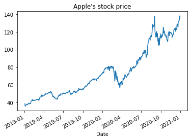
and to plot it using pandas plotting function.
appl_df['Open'].plot(title="Apple's stock price")

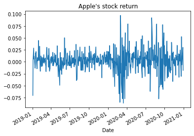
here we covert the stock price to daily stock returns and to plot it
appl_df['Open']=appl_df['Open'].pct_change()
appl_df['Open'].plot(title="Apple's stock return")

From previous experience with deep learning models, we know that we have to scale our data for optimal performance. In our case, we’ll use Scikit- Learn’s StandardScaler and scale our dataset to numbers between zero and one.
sc = StandardScaler()
here we create a univariate pre-processor function that does three steps of min max scaling, creating lags, and separating the data to train and test sets for a given time-series.
def preproc( data, lag, ratio):
    data=data.dropna().iloc[:, 0:1]
    Dates=data.index.unique()
    data.iloc[:, 0] = sc.fit_transform(data.iloc[:, 0].values.reshape(-1, 1))
    for s in range(1, lag):
        data['shift_{}'.format(s)] = data.iloc[:, 0].shift(s)
    X_data = data.dropna().drop(['Open'], axis=1)
    y_data = data.dropna()[['Open']]
    index=int(round(len(X_data)*ratio))
    X_data_train=X_data.iloc[:index,:]
    X_data_test =X_data.iloc[index+1:,:]
    y_data_train=y_data.iloc[:index,:]
    y_data_test =y_data.iloc[index+1:,:]
    return X_data_train,X_data_test,y_data_train,y_data_test,Dates;
Then we apply the univariate pre-processing to the Apple data
a,b,c,d,e=preproc(appl_df, 25, 0.90)
in order to run the models data should be transformed to numpy arrays
a = a.values
b= b.values
c = c.values
d = d.values
and properly reshaped for LSTM modeling
X_train_t = a.reshape(a.shape[0], 1, 24)
X_test_t = b.reshape(b.shape[0], 1, 24)
from keras.models import Sequential
from keras.layers import Dense
from keras.layers import LSTM
import keras.backend as K
from keras.callbacks import EarlyStopping
import keras_tuner as kt
from tensorflow.keras.layers import Dropout
from keras_tuner.tuners import RandomSearch
from keras_tuner.engine.hyperparameters import HyperParameters
here we define a simple Sequential model with two LSTM and two dense layers
K.clear_session()
early_stop = EarlyStopping(monitor='loss', patience=1, verbose=1)
model = Sequential()
model.add(LSTM(12, input_shape=(1, 24), return_sequences=True))
model.add(LSTM(6))
model.add(Dense(6))
model.add(Dense(1))
model.compile(loss='mean_squared_error', optimizer='adam')
and fit the model
model.fit(X_train_t, c,
          epochs=100, batch_size=1, verbose=1,
          callbacks=[early_stop])
Epoch 1/100
431/431 [==============================] - 2s 973us/step - loss: 0.9624
Epoch 2/100
431/431 [==============================] - 0s 947us/step - loss: 1.0980
Epoch 3/100
431/431 [==============================] - 0s 947us/step - loss: 0.9530
Epoch 4/100
431/431 [==============================] - 0s 945us/step - loss: 0.8867
Epoch 5/100
431/431 [==============================] - 0s 943us/step - loss: 0.8433
Epoch 6/100
431/431 [==============================] - 0s 942us/step - loss: 0.5886
Epoch 7/100
431/431 [==============================] - 0s 956us/step - loss: 0.6192
Epoch 8/100
431/431 [==============================] - 0s 973us/step - loss: 0.5257
Epoch 9/100
431/431 [==============================] - 0s 957us/step - loss: 0.4120
Epoch 10/100
431/431 [==============================] - 0s 946us/step - loss: 0.3625
Epoch 11/100
431/431 [==============================] - 0s 944us/step - loss: 0.3114
Epoch 12/100
431/431 [==============================] - 0s 943us/step - loss: 0.3296
Epoch 13/100
431/431 [==============================] - 0s 944us/step - loss: 0.2298
Epoch 14/100
431/431 [==============================] - 0s 945us/step - loss: 0.2337
Epoch 15/100
431/431 [==============================] - 0s 945us/step - loss: 0.2314
Epoch 16/100
431/431 [==============================] - 0s 942us/step - loss: 0.2489
Epoch 17/100
431/431 [==============================] - 0s 940us/step - loss: 0.2131
Epoch 18/100
431/431 [==============================] - 0s 943us/step - loss: 0.1688
Epoch 19/100
431/431 [==============================] - 0s 947us/step - loss: 0.1759
Epoch 20/100
431/431 [==============================] - 0s 974us/step - loss: 0.1767
Epoch 21/100
431/431 [==============================] - 0s 1ms/step - loss: 0.1603
Epoch 22/100
431/431 [==============================] - 1s 1ms/step - loss: 0.1526
Epoch 23/100
431/431 [==============================] - 0s 1ms/step - loss: 0.1666
Epoch 24/100
431/431 [==============================] - 0s 945us/step - loss: 0.1575
Epoch 00024: early stopping
This is in contrast to the tuner approach where options for hyper parameters “hp” are specified and passed to the model
def build_model(hp):
    model = Sequential()
    model.add(LSTM(hp.Int('input_unit',min_value=32,max_value=128,step=32),return_sequences=True, input_shape=(1,24)))
    for i in range(hp.Int('n_layers', 1, 10)):
        model.add(LSTM(hp.Int(f'lstm_{i}_units',min_value=32,max_value=128,step=32),return_sequences=True))
    model.add(LSTM(6))
    model.add(Dropout(hp.Float('Dropout_rate',min_value=0,max_value=0.5,step=0.1)))
    model.add(Dense(6))
    model.add(Dropout(hp.Float('Dropout_rate',min_value=0,max_value=0.5,step=0.1)))
    model.add(Dense(1))
    model.compile(loss='mean_squared_error', optimizer='adam',metrics = ['mse'])
    return model
Thereafter the tuner object is defined here we use the RandomSearch but other options are available as well.
tuner= kt.RandomSearch(
        build_model,
        objective='mse',
        max_trials=10,
        executions_per_trial=3
        )
and instead of fitting the model you run the search function on the tuner object.
tuner.search(
        x=X_train_t,
        y=c,
        epochs=20,
        batch_size=128,
        validation_data=(X_test_t,d),
)
Trial 10 Complete [00h 00m 17s]
mse: 0.8778028885523478

Best mse So Far: 0.8115118543306986
Total elapsed time: 00h 02m 14s
INFO:tensorflow:Oracle triggered exit
Once the hyper parameter training is done it is possible to get the best model
best_model = tuner.get_best_models(num_models=1)[0]
information on the architecture
best_model.summary()
Model: "sequential"
_________________________________________________________________
Layer (type)                 Output Shape              Param #
=================================================================
lstm (LSTM)                  (None, 1, 64)             22784
_________________________________________________________________
lstm_1 (LSTM)                (None, 1, 64)             33024
_________________________________________________________________
lstm_2 (LSTM)                (None, 1, 96)             61824
_________________________________________________________________
lstm_3 (LSTM)                (None, 6)                 2472
_________________________________________________________________
dropout (Dropout)            (None, 6)                 0
_________________________________________________________________
dense (Dense)                (None, 6)                 42
_________________________________________________________________
dropout_1 (Dropout)          (None, 6)                 0
_________________________________________________________________
dense_1 (Dense)              (None, 1)                 7
=================================================================
Total params: 120,153
Trainable params: 120,153
Non-trainable params: 0
_________________________________________________________________
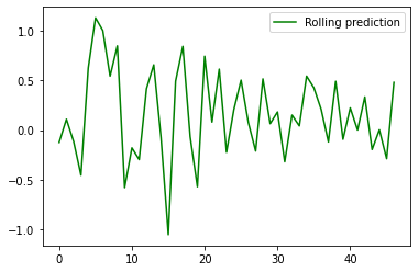
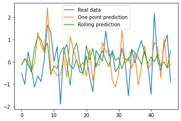
as well as evaluating the performance, here we use the same visualizing approach as discussed in a previous blog post here.
ypredr=[]
st=X_test_t[0].reshape(1, 1, 24)
tmp=st
ptmp=st
val=model.predict(st)
ypredr.append(val.tolist()[0])
for i in range(1, X_test_t.shape[0]):
    tmp=np.append(val, tmp[0,0, 0:-1])
    tmp=tmp.reshape(1, 1, 24)
    ptmp=np.vstack((ptmp,tmp))
    val=model.predict(tmp)
    ypredr.append(val.tolist()[0])
plt.plot(ypredr,color="green", label = "Rolling prediction")
plt.legend()
plt.show()

y_pred = model.predict(X_test_t)
plt.plot(d, label = "Real data")
plt.plot(y_pred, label = "One point prediction")
plt.plot(ypredr, label = "Rolling prediction")
plt.legend()
plt.show()

