Chapter 2 Causal Inference in Practice I: Randomized Controlled Trials and Regression Adjustment

2.1 Introduction

In the first post of this series, we presented a comprehensive overview of key causal inference methods, highlighting the assumptions, strengths, and limitations that distinguish each technique. In this follow-up post, we delve into the two most foundational approaches: Randomized Controlled Trials (RCTs) and Regression Adjustment. Although these methods differ in their reliance on data-generating processes and assumptions, both provide crucial entry points into the logic of causal reasoning. This essay offers a theoretically grounded and practically oriented treatment of each method, including code implementation in R, diagnostics, and interpretive guidance.

RCTs represent the epistemic benchmark for causal inference, often described as the “gold standard” due to their unique ability to eliminate confounding through randomization. Regression Adjustment, by contrast, models the outcome conditional on treatment and covariates, requiring more assumptions but offering wide applicability in observational settings. Despite their differences, both approaches are underpinned by counterfactual reasoning—the idea that causal effects reflect the difference between what actually happened and what would have happened under a different treatment assignment.

Understanding the logic and implementation of these two methods is essential not only for their direct use but also because they serve as the conceptual and statistical scaffolding for more complex techniques such as matching, weighting, and doubly robust estimators.

2.2 1. Randomized Controlled Trials: Design and Analysis

2.2.1 Theoretical Foundations

In an RCT, participants are randomly assigned to treatment or control groups. This process ensures that, on average, both groups are statistically equivalent on all covariates, observed and unobserved. The core assumption is exchangeability—that the potential outcomes are independent of treatment assignment conditional on randomization. This enables simple comparisons of mean outcomes across groups to yield unbiased estimates of causal effects.

Formally, let \(Y(1)\) and \(Y(0)\) denote the potential outcomes under treatment and control, respectively. The average treatment effect (ATE) is defined as:

\[ \text{ATE} = \mathbb{E}[Y(1) - Y(0)] \]

In a perfectly randomized trial, we estimate the ATE by comparing the sample means:

\[ \widehat{\text{ATE}} = \bar{Y}_1 - \bar{Y}_0 \]

This estimator is unbiased and consistent, provided randomization is successfully implemented and compliance is perfect.

2.2.2 R Implementation

Let’s simulate a simple RCT to estimate the effect of a binary treatment on an outcome.

# Load necessary libraries
library(tidyverse)

# Set seed for reproducibility
set.seed(123)

# Simulate data
n <- 1000
data_rct <- tibble(
  treatment = rbinom(n, 1, 0.5),
  outcome = 5 + 2 * treatment + rnorm(n)
)

# Estimate ATE using difference in means
ate_estimate <- data_rct %>%
  group_by(treatment) %>%
  summarise(mean_outcome = mean(outcome)) %>%
  summarise(ATE = diff(mean_outcome))

print(ate_estimate)

2.2.3 Model-Based Inference

While RCTs do not require model-based adjustments, regression models are often used to improve precision or adjust for residual imbalances. In the RCT context, such models are descriptive rather than corrective.

# Linear regression with treatment as predictor
lm_rct <- lm(outcome ~ treatment, data = data_rct)
summary(lm_rct)

The coefficient on the treatment variable in this model provides an estimate of the ATE. Importantly, in randomized designs, the inclusion of additional covariates should not substantially alter the point estimate, though it may reduce variance.

2.2.4 Diagnostics and Integrity

Although randomization ensures internal validity, its practical implementation must be verified. Balance diagnostics, such as standardized mean differences or visualizations of covariate distributions by treatment group, help ensure that the groups are equivalent at baseline. If substantial imbalances exist, especially in small samples, model-based covariate adjustment can improve efficiency but not eliminate bias due to poor randomization.

2.3 2. Regression Adjustment: A Model-Based Approach to Causal Inference

2.3.1 Conceptual Overview

Regression Adjustment, sometimes called covariate adjustment, is one of the most widely used methods for causal estimation in observational studies. Unlike RCTs, this approach requires the assumption of no unmeasured confounding, often called conditional ignorability:

\[ Y(1), Y(0) \perp D \mid X \]

Here, \(D\) is the binary treatment variable and \(X\) is a vector of observed covariates. The central idea is to control for confounders \(X\) that affect both treatment assignment and potential outcomes.

The linear model typically takes the form:

\[ Y = \beta_0 + \beta_1 D + \beta_2 X + \varepsilon \]

The coefficient \(\beta_1\) is interpreted as the average treatment effect, assuming the model is correctly specified and all relevant confounders are included.

2.3.2 R Implementation

We now simulate observational data with a confounder to demonstrate regression adjustment.

# Simulate observational data
set.seed(123)
n <- 1000
x <- rnorm(n)
d <- rbinom(n, 1, plogis(0.5 * x))
y <- 5 + 2 * d + 1.5 * x + rnorm(n)

data_obs <- tibble(
  treatment = d,
  covariate = x,
  outcome = y
)

# Naive model (without adjustment)
lm_naive <- lm(outcome ~ treatment, data = data_obs)
summary(lm_naive)

# Adjusted model
lm_adjusted <- lm(outcome ~ treatment + covariate, data = data_obs)
summary(lm_adjusted)

The naive model, which omits the confounder, yields a biased estimate of the treatment effect. By contrast, the adjusted model corrects this bias, provided all relevant confounders are included and the functional form is correct.

2.3.3 Limitations and Diagnostics

Regression Adjustment hinges on correct model specification and the inclusion of all relevant confounders. Omitted variable bias remains a major threat, and multicollinearity or misspecified functional forms can distort estimates. Residual plots, variance inflation factors, and specification tests are essential for model diagnostics.

Moreover, regression does not address overlap—the requirement that all units have a non-zero probability of receiving each treatment conditional on covariates. Violations of this assumption can lead to extrapolation and poor generalizability.

One strategy to assess covariate overlap is to model the propensity score and visualize its distribution across treatment groups.

# Estimate propensity scores
ps_model <- glm(treatment ~ covariate, data = data_obs, family = binomial())
data_obs <- data_obs %>% mutate(pscore = predict(ps_model, type = "response"))

# Plot propensity scores
ggplot(data_obs, aes(x = pscore, fill = factor(treatment))) +
  geom_density(alpha = 0.5) +
  labs(fill = "Treatment Group", title = "Propensity Score Overlap")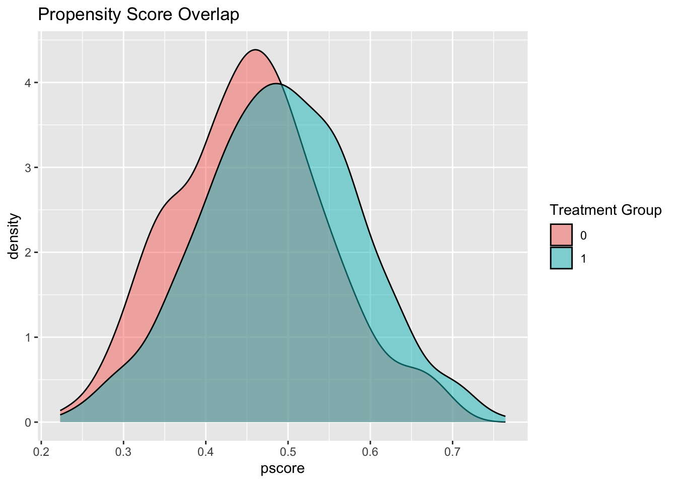

If there is poor overlap between groups, regression adjustment may yield estimates with high variance and questionable validity.

2.3.4 Causal Interpretation

While regression models provide estimates of conditional treatment effects, care must be taken in interpreting these coefficients causally. The treatment effect estimated by regression adjustment is unbiased only under strong assumptions: no unmeasured confounding, correct model specification, and sufficient overlap.

This makes regression adjustment a double-edged sword. Its ease of use and interpretability make it appealing, but its susceptibility to hidden bias requires rigorous scrutiny.

2.4 Toward Integrated Reasoning

The juxtaposition of RCTs and regression adjustment highlights the contrast between design-based and model-based inference. RCTs achieve causal identification through the randomization mechanism itself, rendering statistical adjustment unnecessary (but sometimes helpful for precision). Regression adjustment, on the other hand, relies entirely on the plausibility of its assumptions, making it vulnerable to hidden confounding and specification errors.

Importantly, these methods should not be viewed in isolation. Hybrid designs and analytic strategies—such as regression adjustment in RCTs or design-based diagnostics in observational studies—blur the boundaries and point toward more integrated approaches to causal inference.

Furthermore, emerging methods such as doubly robust estimation, propensity score weighting, and machine learning–based causal estimators build upon the foundations established by these two methods. Understanding the mechanics and logic of RCTs and regression adjustment is thus a prerequisite for mastering more advanced techniques.

2.5 Conclusion

In this installment, we explored the theoretical rationale, implementation, and practical considerations of two cornerstone methods in causal inference: Randomized Controlled Trials and Regression Adjustment. RCTs provide unmatched causal credibility when feasible, while regression models offer flexible tools for analyzing observational data under strong assumptions. Their complementary roles in the causal inference toolkit make them indispensable for any applied researcher.

The next entry in this series will turn to Propensity Score Methods, where we will examine how matching and weighting strategies seek to approximate randomized experiments using observational data. As with all causal methods, the key lies not just in computation, but in the clarity of assumptions and the integrity of reasoning.

By combining design principles, diagnostic rigor, and ethical sensitivity, causal inference offers a powerful framework for navigating the complexity of real-world data.