Chapter 4 Model-Free Reinforcement Learning: Temporal Difference and Monte Carlo Methods in R
4.1 Introduction
In many real-world decision-making problems, the environment model—comprising transition probabilities and reward functions—is unknown or too complex to specify explicitly. Model-free reinforcement learning (RL) methods address this by learning optimal policies directly from experience, without requiring full knowledge of the underlying Markov Decision Process (MDP). Two foundational model-free methods are Temporal Difference (TD) learning and Monte Carlo (MC) methods. TD learning updates value estimates online using one-step lookahead and bootstrapping, while MC methods learn from complete episodes by averaging returns. This post presents these approaches with mathematical intuition, R implementations, and an illustrative environment. We also compare how learned policies adapt—or fail to adapt—when rewards change after training, illuminating the distinction between goal-directed and habitual learning.
Suppose an agent interacts with an environment defined by states \(S\), actions \(A\), and a discount factor \(\gamma \in [0,1]\). The goal is to learn the action-value function \(Q^\pi(s,a)\), the expected discounted return starting from state \(s\), taking action \(a\), and following policy \(\pi\) thereafter: \[Q^\pi(s,a) = \mathbb{E}_\pi \left[ \sum_{t=0}^\infty \gamma^t R_{t+1} \mid S_0 = s, A_0 = a \right]\]
Q-Learning is an off-policy TD control method that updates the estimate \(Q(s,a)\) incrementally after each transition: \[Q(s,a) \leftarrow Q(s,a) + \alpha \left( r + \gamma \max_{a'} Q(s', a') - Q(s,a) \right)\] where \(\alpha\) is the learning rate, \(r\) the reward received, and \(s'\) the next state. This update bootstraps using the current estimate of \(Q\) at \(s'\).
Monte Carlo methods learn \(Q\) by averaging returns observed after visiting \((s,a)\). Every-visit MC estimates \(Q\) by averaging the total discounted return \(G_t\) following each occurrence of \((s,a)\) within complete episodes: \[Q(s,a) \approx \frac{1}{N(s,a)} \sum_{i=1}^{N(s,a)} G_t^{(i)}\] where \(N(s,a)\) is the count of visits to \((s,a)\) and \(G_t^{(i)}\) is the return following the \(i\)-th visit.
4.2 Implementation
- Step 1: Defining the Environment
We use a 10-state, 2-action environment with stochastic transitions and rewards:
# Common settings
n_states <- 10
n_actions <- 2
gamma <- 0.9
terminal_state <- n_states

# Environment: transition + reward models
set.seed(42)
transition_model <- array(0, dim = c(n_states, n_actions, n_states))
reward_model <- array(0, dim = c(n_states, n_actions, n_states))

for (s in 1:(n_states - 1)) {
  # Action 1: 90% to next state, 10% to random state
  transition_model[s, 1, s + 1] <- 0.9
  rand_state_1 <- sample(1:n_states, 1)
  transition_model[s, 1, rand_state_1] <- transition_model[s, 1, rand_state_1] + 0.1

  # Action 2: 80% and 20% to random states
  rand_states_2 <- sample(1:n_states, 2, replace = TRUE)
  transition_model[s, 2, rand_states_2[1]] <- transition_model[s, 2, rand_states_2[1]] + 0.8
  transition_model[s, 2, rand_states_2[2]] <- transition_model[s, 2, rand_states_2[2]] + 0.2

  # Rewards
  for (s_prime in 1:n_states) {
    reward_model[s, 1, s_prime] <- ifelse(s_prime == n_states, 1.0, 0.1 * runif(1))
    reward_model[s, 2, s_prime] <- ifelse(s_prime == n_states, 0.5, 0.05 * runif(1))
  }
}

# Terminal state
transition_model[n_states, , ] <- 0
reward_model[n_states, , ] <- 0

# Sampling function
sample_env <- function(s, a) {
  probs <- transition_model[s, a, ]
  s_prime <- sample(1:n_states, 1, prob = probs)
  reward <- reward_model[s, a, s_prime]
  list(s_prime = s_prime, reward = reward)
}
This environment simulates stochastic state transitions where action 1 favors forward progress with higher terminal reward, while action 2 introduces more randomness with lower terminal reward.
- Step 2: Q-Learning Implementation
The Q-Learning function runs episodes, selects actions using \(\epsilon\)-greedy exploration, and updates Q-values using the TD rule:
q_learning <- function(episodes = 1000, alpha = 0.1, epsilon = 0.1) {
  Q <- matrix(0, nrow = n_states, ncol = n_actions)

  for (ep in 1:episodes) {
    s <- 1
    while (TRUE) {
      # Epsilon-greedy action selection
      if (runif(1) < epsilon) {
        a <- sample(1:n_actions, 1)
      } else {
        a <- which.max(Q[s, ])
      }

      out <- sample_env(s, a)
      s_prime <- out$s_prime
      reward <- out$reward

      # TD update
      Q[s, a] <- Q[s, a] + alpha * (reward + gamma * max(Q[s_prime, ]) - Q[s, a])

      if (s_prime == n_states) break
      s <- s_prime
    }
  }

  apply(Q, 1, which.max)
}

# Train Q-Learning
ql_policy_before <- q_learning()
print(ql_policy_before)
## [1] 1 2 2 2 1 1 1 1 1 1- Step 3: Monte Carlo Every-Visit Implementation
This MC method generates complete episodes and updates \(Q\) by averaging discounted returns for every visit of \((s,a)\):
monte_carlo <- function(episodes = 1000, epsilon = 0.1) {
  Q <- matrix(0, nrow = n_states, ncol = n_actions)
  returns <- vector("list", n_states * n_actions)
  names(returns) <- paste(rep(1:n_states, each = n_actions),
                          rep(1:n_actions, n_states), sep = "_")

  for (ep in 1:episodes) {
    episode <- list()
    s <- 1

    # Generate episode
    while (TRUE) {
      if (runif(1) < epsilon) {
        a <- sample(1:n_actions, 1)
      } else {
        a <- which.max(Q[s, ])
      }

      out <- sample_env(s, a)
      episode[[length(episode) + 1]] <- list(state = s, action = a, reward = out$reward)

      if (out$s_prime == n_states) break
      s <- out$s_prime
    }

    # Compute returns backward
    G <- 0
    for (t in length(episode):1) {
      s <- episode[[t]]$state
      a <- episode[[t]]$action
      r <- episode[[t]]$reward
      G <- gamma * G + r

      key <- paste(s, a, sep = "_")
      returns[[key]] <- c(returns[[key]], G)
      Q[s, a] <- mean(returns[[key]])
    }
  }

  apply(Q, 1, which.max)
}

# Train Monte Carlo
mc_policy_before <- monte_carlo()
print(mc_policy_before)
## [1] 1 2 1 2 2 1 1 1 1 1- Step 4: Simulating Outcome Devaluation
We now alter the environment by removing the terminal reward, simulating devaluation:
# Devalue terminal reward
for (s in 1:(n_states - 1)) {
  reward_model[s, 1, n_states] <- 0
  reward_model[s, 2, n_states] <- 0
}- Step 5: Dynamic Programming for Comparison
First, we implement value iteration to represent model-based learning:
value_iteration <- function(theta = 0.001, max_iter = 1000) {
  V <- numeric(n_states)

  for (iter in 1:max_iter) {
    delta <- 0
    for (s in 1:(n_states - 1)) {
      v <- V[s]
      action_values <- numeric(n_actions)

      for (a in 1:n_actions) {
        action_values[a] <- sum(transition_model[s, a, ] *
          (reward_model[s, a, ] + gamma * V))
      }

      V[s] <- max(action_values)
      delta <- max(delta, abs(v - V[s]))
    }

    if (delta < theta) break
  }

  # Extract policy
  policy <- numeric(n_states)
  for (s in 1:(n_states - 1)) {
    action_values <- numeric(n_actions)
    for (a in 1:n_actions) {
      action_values[a] <- sum(transition_model[s, a, ] *
        (reward_model[s, a, ] + gamma * V))
    }
    policy[s] <- which.max(action_values)
  }

  policy
}

# Compute policies before devaluation
dp_policy_before <- value_iteration()
Now we compare policies after devaluation. DP recomputes with new rewards, while Q-Learning and Monte Carlo maintain their learned policies without retraining:
# DP recomputes with new rewards
dp_policy_after <- value_iteration()

# Q-learning and MC keep previous policy (habitual)
ql_policy_after <- ql_policy_before
mc_policy_after <- mc_policy_before- Step 6: Visualizing the Policies
plot_policy <- function(policy, label, col = "skyblue") {
  barplot(policy, names.arg = 1:n_states, col = col,
          ylim = c(0, 3), ylab = "Action (1=A1, 2=A2)",
          main = label, las = 1)
  abline(h = 1.5, lty = 2, col = "gray")
}

par(mfrow = c(3, 2), mar = c(4, 4, 2, 1))
plot_policy(dp_policy_before, "DP Policy Before")
plot_policy(dp_policy_after, "DP Policy After", "lightgreen")
plot_policy(ql_policy_before, "Q-Learning Policy Before")
plot_policy(ql_policy_after, "Q-Learning Policy After", "orange")
plot_policy(mc_policy_before, "MC Policy Before")
plot_policy(mc_policy_after, "MC Policy After", "orchid")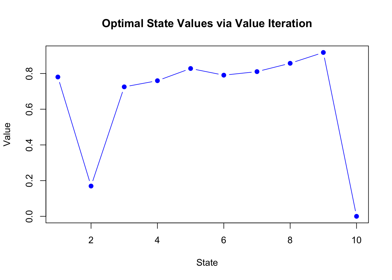
4.3 Interpretation and Discussion
Dynamic Programming adapts immediately after devaluation because it recalculates the policy using the updated reward model. In contrast, Q-Learning and Monte Carlo methods, which learn from past experience, maintain their prior policies unless explicitly retrained. This reflects habitual behavior—a policy learned from experience that does not flexibly adjust to changed outcomes without further learning.
This illustrates a core difference: model-based methods (like DP) support goal-directed behavior, recomputing optimal decisions as the environment changes, while model-free methods (like Q-Learning and MC) support habitual behavior, relying on cached values learned from past rewards.
Temporal Difference and Monte Carlo methods provide powerful approaches to reinforcement learning when the environment is unknown. TD learning’s bootstrapping allows online updates after each transition, while Monte Carlo averages full returns after complete episodes. Both learn policies from experience rather than models. Understanding their differences—particularly in terms of bias-variance tradeoffs and adaptability—is crucial for selecting the right approach for specific problems.
| Aspect | Monte Carlo | Q-Learning (TD) |
|---|---|---|
| Learning | Learns from complete episodes | Learns after each transition |
| Update Rule | \(Q(s,a) \approx \frac{1}{N(s,a)} \sum G_t^{(i)}\) | \(Q(s,a) \leftarrow Q(s,a) + \alpha [r + \gamma \max_{a'} Q(s', a') - Q(s,a)]\) |
| Episodes | Requires complete episodes | Works with incomplete episodes |
| Bias-Variance | Unbiased, high variance | Biased (bootstrapping), low variance |
| Policy Type | On-policy (typically) | Off-policy |
| Efficiency | Less efficient (waits for completion) | More efficient (immediate updates) |
| Adaptation | Slow without retraining | Faster with incremental updates |