Chapter 4 Nonlinear Dynamics in One Dimension
You’re watching bacteria under a microscope. At first, the population doubles every twenty minutes—classic exponential growth. But as the petri dish fills, something curious happens. The doubling slows, then stops. The population doesn’t collapse; it stabilizes at some maximum level, fluctuating gently around equilibrium.
This isn’t a failure of the exponential model—it’s the emergence of something richer: nonlinear dynamics. Where linear equations gave us predictable exponential curves, nonlinear equations reveal systems that can settle into equilibrium, oscillate between states, or exhibit behavior so complex it appears random.
In our previous post, we conquered separable differential equations using separation of variables. We learned to predict when hot chocolate reaches drinking temperature and how salt accumulates in mixing tanks. But those examples shared a crucial limitation: they were fundamentally linear in their dependent variables. Today, we venture into the fascinating world of nonlinear dynamics.
4.1 When More Becomes Different
Consider our bacterial population again. The exponential model \(\frac{dN}{dt} = rN\) works perfectly when resources are unlimited. But real bacteria compete for space and nutrients. As density increases, growth rate decreases.
The simplest model capturing this is the logistic equation:
\[\frac{dN}{dt} = rN\left(1 - \frac{N}{K}\right)\]
Here, \(r\) is the intrinsic growth rate and \(K\) is the carrying capacity—the maximum population the environment can sustain.
This innocent-looking equation exhibits behavior impossible in linear systems. When \(N\) is small compared to \(K\), the term \((1 - N/K) \approx 1\), and we recover exponential growth. But as \(N\) approaches \(K\), growth slows to zero.
Unlike our previous equations, the logistic equation reveals something profound about equilibrium. Where do populations settle? What happens if we disturb them? These questions lead us to fixed points and stability.
4.2 Finding the Balance Points
For any differential equation \(\frac{dx}{dt} = f(x)\), fixed points (or equilibrium points) occur where the rate of change equals zero:
\[f(x^*) = 0\]
These are values where the system stops changing—points of equilibrium.
For the logistic equation:
\[rN\left(1 - \frac{N}{K}\right) = 0\]
This gives two fixed points:
- \(N^* = 0\) (extinction)
- \(N^* = K\) (carrying capacity)
But knowing where equilibria exist isn’t enough. We need to understand their stability. If we slightly perturb the system from equilibrium, does it return or drift away?
The key insight: examine the derivative of \(f(x)\) at the fixed point. For \(f'(x^*) < 0\), small perturbations decay back to equilibrium—the fixed point is stable. For \(f'(x^*) > 0\), perturbations grow away—the fixed point is unstable.
Let’s check our logistic fixed points. With \(f(N) = rN(1 - N/K)\):
\[f'(N) = r\left(1 - \frac{2N}{K}\right)\]
At \(N^* = 0\): \(f'(0) = r > 0\) (unstable—a small population will grow)
At \(N^* = K\): \(f'(K) = -r < 0\) (stable—populations near carrying capacity return to it)
4.3 The Logistic Portrait
Let’s visualize this behavior:
##
## Attaching package: 'gridExtra'
## The following object is masked from 'package:dplyr':
##
## combine# Parameters for logistic growth
r <- 0.5
K <- 100
# Define the logistic function
logistic <- function(N) r * N * (1 - N/K)
# Phase portrait data
N_vals <- seq(0, 120, by = 1)
phase_data <- data.frame(
N = N_vals,
dN_dt = logistic(N_vals)
)
# Analytical solution for trajectories
logistic_solution <- function(t, N0, r, K) {
K / (1 + ((K - N0) / N0) * exp(-r * t))
}
# Generate trajectory data for different initial conditions
time <- seq(0, 20, by = 0.1)
initial_conditions <- c(5, 25, 75, 110)
trajectory_data <- do.call(rbind, lapply(initial_conditions, function(N0) {
data.frame(
time = time,
N = logistic_solution(time, N0, r, K),
initial = paste0("N₀ = ", N0)
)
}))
# Phase portrait
phase_plot <- ggplot(phase_data, aes(x = N, y = dN_dt)) +
geom_line(color = "steelblue", linewidth = 1.2) +
geom_hline(yintercept = 0, linetype = "dashed", alpha = 0.7) +
geom_vline(xintercept = c(0, K), linetype = "dashed", alpha = 0.7, color = "red") +
geom_point(data = data.frame(x = c(0, K), y = c(0, 0),
type = c("Unstable", "Stable")),
aes(x = x, y = y, color = type), size = 3) +
scale_color_manual(values = c("Unstable" = "red", "Stable" = "darkgreen")) +
annotate("text", x = 5, y = 2, label = "Unstable", color = "red") +
annotate("text", x = K - 5, y = -2, label = "Stable", color = "darkgreen") +
labs(
title = "Phase Portrait: Logistic Growth",
x = "Population (N)",
y = "Growth Rate (dN/dt)",
subtitle = "Fixed points and flow direction"
) +
theme_minimal() +
theme(legend.position = "none") +
coord_cartesian(xlim = c(0, 120))
# Trajectory plot
trajectory_plot <- ggplot(trajectory_data, aes(x = time, y = N, color = initial)) +
geom_line(linewidth = 1) +
geom_hline(yintercept = K, linetype = "dashed", alpha = 0.7) +
annotate("text", x = 15, y = K + 5, label = paste("Carrying Capacity =", K)) +
labs(
title = "Solution Trajectories",
x = "Time",
y = "Population (N)",
color = "Initial Condition",
subtitle = "All trajectories converge to carrying capacity"
) +
theme_minimal() +
theme(legend.position = "bottom")
grid.arrange(phase_plot, trajectory_plot, ncol = 1)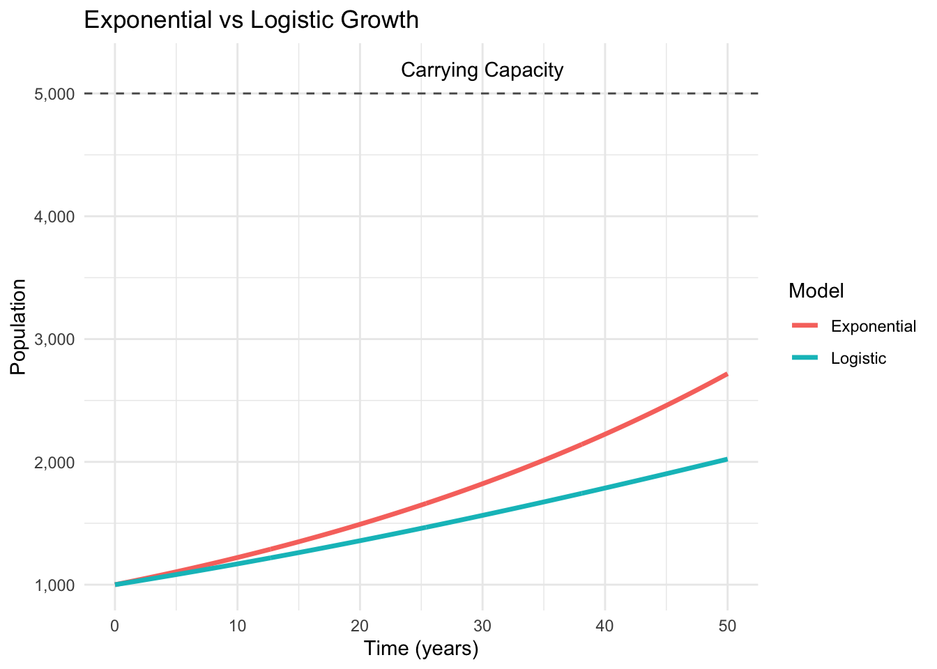
The phase portrait (top) shows how growth rate varies with population size. The arrows indicate flow direction—where populations move over time. Notice how all arrows point toward the stable fixed point at \(N = K\).
The trajectory plot (bottom) reveals the S-shaped logistic curve familiar from biology. Regardless of initial conditions, all populations eventually settle at carrying capacity.
4.4 Beyond Simple Equilibrium: Bistable Systems
Not all nonlinear systems are as well-behaved. Consider a more complex ecological scenario where a population faces an Allee effect—individuals struggle when density is too low (perhaps they can’t find mates or defend against predators effectively).
A simple model:
\[\frac{dN}{dt} = rN\left(\frac{N}{A} - 1\right)\left(1 - \frac{N}{K}\right)\]
where \(A\) is the Allee threshold—populations below this level decline toward extinction.
Setting the right side to zero gives three fixed points:
- \(N^* = 0\) (extinction)
- \(N^* = A\) (Allee threshold)
- \(N^* = K\) (carrying capacity)
For stability, we determine the sign of \(\frac{dN}{dt}\) between fixed points:
- For \(0 < N < A\): \(\frac{dN}{dt} < 0\) (population declines)
- For \(A < N < K\): \(\frac{dN}{dt} > 0\) (population grows)
- For \(N > K\): \(\frac{dN}{dt} < 0\) (population declines)
This creates a bistable system: populations either go extinct (if they start below \(A\)) or survive at carrying capacity (if they start above \(A\)). The Allee threshold is an unstable equilibrium—a knife-edge balance where the slightest push determines fate.
# Parameters for Allee effect
r <- 0.3
A <- 30
K <- 100

# Define the Allee function
allee <- function(N) r * N * (N/A - 1) * (1 - N/K)

# Phase portrait data
N_vals <- seq(0, 120, by = 0.5)
allee_phase_data <- data.frame(
  N = N_vals,
  dN_dt = allee(N_vals)
)

# Numerical solution using Euler's method
solve_allee <- function(N0, time_span = 30, dt = 0.1) {
  times <- seq(0, time_span, by = dt)
  N <- numeric(length(times))
  N[1] <- N0

  for (i in 2:length(times)) {
    dN <- dt * allee(N[i-1])
    N[i] <- max(0, N[i-1] + dN)  # Prevent negative populations
  }

  data.frame(time = times, N = N)
}

# Generate trajectories
initial_conditions_allee <- c(10, 25, 35, 80)

allee_trajectory_data <- do.call(rbind, lapply(initial_conditions_allee, function(N0) {
  temp_data <- solve_allee(N0)
  temp_data$initial <- paste0("N₀ = ", N0)
  temp_data
}))

# Phase portrait
allee_phase_plot <- ggplot(allee_phase_data, aes(x = N, y = dN_dt)) +
  geom_line(color = "purple", linewidth = 1.2) +
  geom_hline(yintercept = 0, linetype = "dashed", alpha = 0.7) +
  geom_vline(xintercept = c(0, A, K), linetype = "dashed", alpha = 0.7, color = "red") +
  geom_point(data = data.frame(x = c(0, A, K), y = c(0, 0, 0),
                               type = c("Stable", "Unstable", "Stable")),
             aes(x = x, y = y, color = type), size = 3) +
  scale_color_manual(values = c("Unstable" = "red", "Stable" = "darkgreen")) +
  annotate("text", x = 5, y = -1, label = "Stable", color = "darkgreen", size = 3) +
  annotate("text", x = A, y = 1, label = "Unstable", color = "red", size = 3) +
  annotate("text", x = K, y = -1, label = "Stable", color = "darkgreen", size = 3) +
  labs(
    title = "Bistable System: Allee Effect",
    x = "Population (N)",
    y = "Growth Rate (dN/dt)",
    subtitle = "Two stable states separated by unstable threshold"
  ) +
  theme_minimal() +
  theme(legend.position = "none") +
  coord_cartesian(xlim = c(0, 120))

# Trajectory plot
allee_trajectory_plot <- ggplot(allee_trajectory_data, aes(x = time, y = N, color = initial)) +
  geom_line(linewidth = 1) +
  geom_hline(yintercept = c(A, K), linetype = "dashed", alpha = 0.7) +
  annotate("text", x = 20, y = A + 3, label = paste("Allee Threshold =", A)) +
  annotate("text", x = 20, y = K + 3, label = paste("Carrying Capacity =", K)) +
  labs(
    title = "Bistable Dynamics",
    x = "Time",
    y = "Population (N)",
    color = "Initial Condition",
    subtitle = "Fate depends on initial population size"
  ) +
  theme_minimal() +
  theme(legend.position = "bottom")

grid.arrange(allee_phase_plot, allee_trajectory_plot, ncol = 1)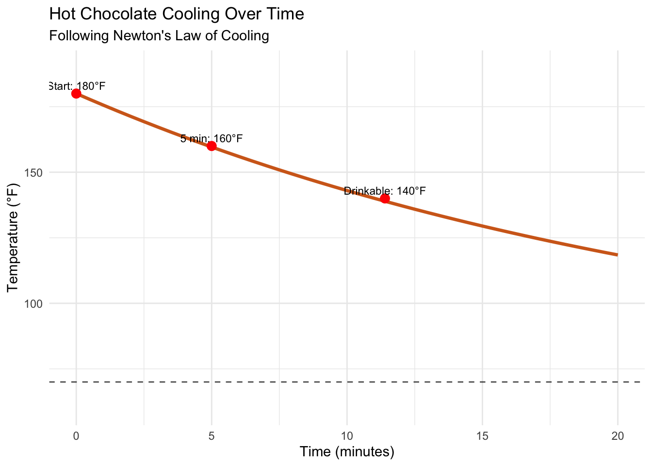
The bistable system reveals something profound: history matters. Two identical environments can end up in completely different states depending on their past. A population starting at \(N_0 = 25\) goes extinct, while one at \(N_0 = 35\) thrives—a difference of just 10 individuals determines survival or extinction.
This sensitivity appears throughout ecology, economics, and social systems. Markets can settle into high-trust or low-trust equilibria. Lakes can remain clear or become turbid. Social movements can fizzle out or reach critical mass.
4.5 The Geometry of Dynamics
Working with nonlinear differential equations requires developing geometric intuition. The phase portrait—a plot of \(\frac{dx}{dt}\) versus \(x\)—reveals the system’s complete behavioral repertoire at a glance.
Key features to look for:
Fixed Points: Where the curve crosses the horizontal axis (\(\frac{dx}{dt} = 0\))
Stability: Determined by the slope at fixed points. Negative slopes indicate stability (arrows point toward the fixed point), positive slopes indicate instability (arrows point away)
Flow Direction: Above the axis, \(\frac{dx}{dt} > 0\), so \(x\) increases (rightward flow). Below the axis, \(\frac{dx}{dt} < 0\), so \(x\) decreases (leftward flow)
Basins of Attraction: Regions of initial conditions leading to the same long-term fate. In bistable systems, these basins are separated by unstable fixed points
This geometric perspective transforms equation-solving into pattern recognition. Complex dynamics become visible as landscapes of hills (unstable points) and valleys (stable points), with trajectories flowing downhill according to the system’s internal logic.
4.6 Harvesting and Catastrophic Collapse
Let’s explore a darker application: what happens when we harvest a population governed by logistic growth? Suppose we remove individuals at constant rate \(h\):
\[\frac{dN}{dt} = rN\left(1 - \frac{N}{K}\right) - h\]
For small harvest rates, this seems manageable—just reduce the equilibrium population slightly. But nonlinear systems can surprise us.
The fixed points satisfy:
\[rN^*\left(1 - \frac{N^*}{K}\right) - h = 0\]
This is a quadratic equation. Using the quadratic formula:
\[N^* = \frac{K}{2}\left(1 \pm \sqrt{1 - \frac{4h}{rK}}\right)\]
For real solutions, we need:
\[1 - \frac{4h}{rK} \geq 0\]
This gives a critical harvest rate:
\[h_{\text{crit}} = \frac{rK}{4}\]
For \(h < h_{\text{crit}}\), we have two fixed points. For \(h > h_{\text{crit}}\), no equilibrium exists—any harvest rate exceeding this threshold drives the population to extinction regardless of initial conditions.
# Parameters for harvesting model
r <- 0.5
K <- 100
h_values <- c(5, 10, 12.5, 15)
h_crit <- r * K / 4  # Critical harvest rate = 12.5

# Create phase portraits for different harvest rates
harvesting_plots <- lapply(h_values, function(h) {
  harvesting <- function(N) r * N * (1 - N/K) - h

  N_vals <- seq(0, 120, by = 1)
  phase_data <- data.frame(
    N = N_vals,
    dN_dt = harvesting(N_vals)
  )

  # Calculate fixed points if they exist
  fixed_points <- NULL
  if (h <= h_crit) {
    discriminant <- sqrt(1 - 4*h/(r*K))
    N_fixed1 <- (K/2) * (1 - discriminant)
    N_fixed2 <- (K/2) * (1 + discriminant)
    fixed_points <- data.frame(
      x = c(N_fixed1, N_fixed2),
      y = c(0, 0),
      type = c("Unstable", "Stable")
    )
  }

  p <- ggplot(phase_data, aes(x = N, y = dN_dt)) +
    geom_line(color = "steelblue", linewidth = 1) +
    geom_hline(yintercept = 0, linetype = "dashed", alpha = 0.7) +
    labs(
      title = paste("Harvest Rate h =", h),
      x = "Population (N)",
      y = "dN/dt",
      subtitle = ifelse(h <= h_crit, "Sustainable", "Population Collapse")
    ) +
    theme_minimal() +
    coord_cartesian(xlim = c(0, 120), ylim = c(-15, 15))

  if (!is.null(fixed_points)) {
    p <- p + geom_point(data = fixed_points, aes(x = x, y = y, color = type), size = 2) +
      scale_color_manual(values = c("Unstable" = "red", "Stable" = "darkgreen")) +
      theme(legend.position = "none")
  }

  p
})

do.call(grid.arrange, c(harvesting_plots, ncol = 2))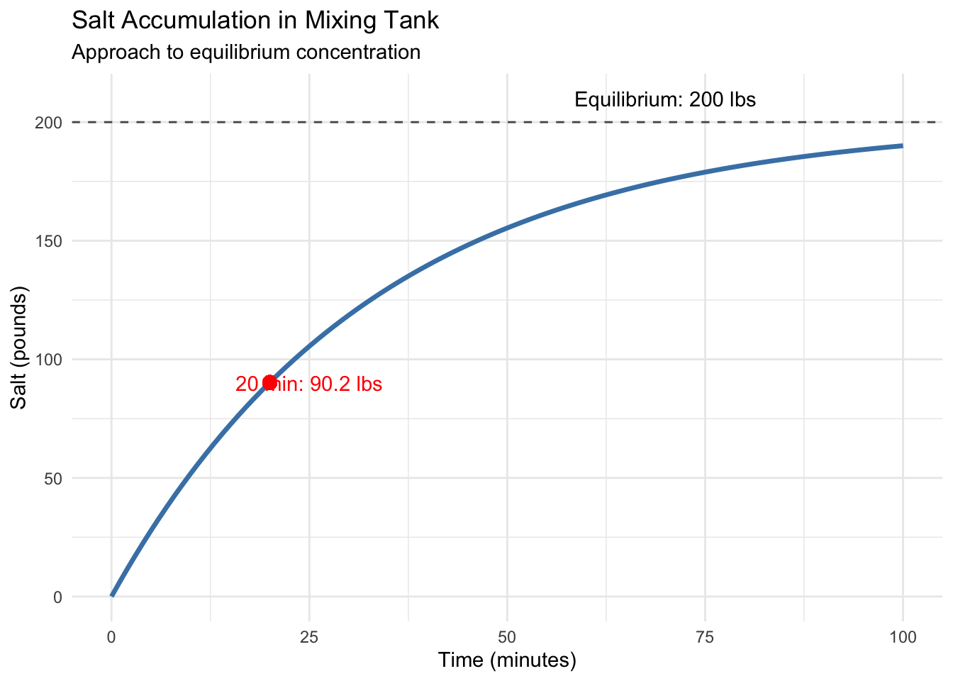
The harvesting model reveals how nonlinear systems exhibit catastrophic collapse—sudden transitions from stable to unstable states as parameters cross critical thresholds. Below the critical harvest rate, the population settles into a reduced but sustainable equilibrium. Above it, no equilibrium exists, and the population inevitably crashes.
This threshold behavior appears throughout complex systems. Coral reefs suddenly bleach when ocean temperatures exceed critical values. Financial markets can transition rapidly from stable to chaotic. Climate systems may have tipping points beyond which feedback loops drive irreversible change.
4.7 The Richness of One Dimension
Even in one dimension, nonlinear differential equations reveal remarkable complexity. We’ve seen systems with multiple equilibria, threshold effects, and catastrophic transitions. But we’ve only scratched the surface.
Consider the equation:
\[\frac{dx}{dt} = x^3 - x\]
This simple cubic produces three fixed points: \(x^* = -1, 0, 1\). The outer points are stable, the center point unstable, creating another bistable system. Small changes in initial conditions near \(x = 0\) determine whether the system settles at \(x = -1\) or \(x = 1\).
Or the transcendental equation:
\[\frac{dx}{dt} = \sin(x) - \gamma\]
For \(\gamma < 1\), this system has multiple stable and unstable fixed points, creating a landscape of alternating attraction and repulsion. As \(\gamma\) increases toward 1, stable and unstable points approach each other, eventually colliding and disappearing in what mathematicians call a saddle-node bifurcation.
These phenomena—bistability, thresholds, bifurcations—emerge naturally from nonlinear dynamics. They’re not mathematical curiosities but fundamental features of complex systems.
4.8 Building Intuition for the Nonlinear World
Working with nonlinear equations develops a different kind of mathematical intuition. Where linear thinking emphasizes proportionality and superposition, nonlinear thinking recognizes thresholds, feedback loops, and emergent behavior.
Key insights:
Small Changes, Big Effects: Tiny differences in initial conditions or parameters can lead to dramatically different outcomes
Multiple Equilibria: Complex systems often have more than one stable state. Which emerges depends on history and initial conditions
Thresholds Matter: Many systems exhibit critical values—cross them and behavior changes qualitatively
Stability is Local: A system might be stable to small perturbations but unstable to large ones
These principles appear across disciplines. Population ecologists study tipping points in ecosystem collapse. Economists analyze multiple equilibria in markets. Climate scientists investigate threshold effects in global warming. Neuroscientists examine bistable states in neural networks.
4.9 The Path Forward
We’ve explored the rich behavior possible in one-dimensional nonlinear systems—from simple logistic growth to bistable dynamics and catastrophic collapse. We’ve learned to read phase portraits like maps, identifying stable valleys and unstable peaks in the landscape of dynamics.
But the real world is rarely one-dimensional. Predators interact with prey, diseases spread through populations, and chemical reactions involve multiple species. In our next post, we’ll extend these concepts to systems of differential equations, where multiple variables change simultaneously, each influencing the others.
We’ll discover that two-dimensional systems can exhibit behaviors impossible in one dimension: closed orbital trajectories, limit cycles, and strange attractors. We’ll explore the famous Lotka-Volterra predator-prey model and see how competition between species creates complex dynamics.
The mathematical techniques you’ve learned today—finding fixed points, analyzing stability, reading phase portraits—form the foundation for understanding these multi-dimensional systems. Every complex system, no matter how many variables it contains, can be understood by building up from these basic concepts.
The world is nonlinear, and now you have the tools to read its hidden patterns.