Chapter 3 Solving Simple Differential Equations
You’re sitting in a café, watching steam rise from your hot chocolate. The barista mentions it was made at 180°F, and you wonder: when will it cool to a comfortable 140°F? This isn’t just idle curiosity—it’s a differential equation waiting to be solved.
In our previous post, we explored how differential equations describe the world around us. We saw the mathematical structures that govern cooling coffee, growing populations, and radioactive decay. But recognizing these patterns is only half the story. Today, we’ll learn how to solve them.
The good news is that many differential equations yield to surprisingly straightforward techniques. The better news is that once you master these methods, you’ll have tools powerful enough to predict the future—at least for systems that follow predictable rules.
3.1 The Art of Separation
Let’s return to that hot chocolate. Newton’s law of cooling tells us:
\[\frac{dT}{dt} = -k(T - T_{room})\]
where \(T(t)\) is temperature at time \(t\), \(k\) is a cooling constant, and \(T_{room}\) is room temperature (say, 70°F).
This equation belongs to a family called separable differential equations. These have the special property that we can separate the variables—getting all the \(T\) terms on one side and all the \(t\) terms on the other. The general form looks like:
\[\frac{dy}{dx} = g(x)h(y)\]
Notice how the right side factors into a function of \(x\) times a function of \(y\). This separation is what makes these equations solvable using basic calculus.
For our cooling chocolate, let’s substitute \(u = T - T_{room}\), so \(\frac{du}{dt} = \frac{dT}{dt}\). Our equation becomes:
\[\frac{du}{dt} = -ku\]
This is separable! We can rewrite it as:
\[\frac{du}{u} = -k , dt\]
Now we integrate both sides. The left side gives us \(\ln|u|\), and the right side gives us \(-kt + C\):
\[\ln|u| = -kt + C\]
Exponentiating both sides:
\[u = e^{-kt + C} = e^C \cdot e^{-kt}\]
Since \(e^C\) is just a constant (let’s call it \(A\)), we have:
\[u = A e^{-kt}\]
Substituting back: \(T - T_{room} = A e^{-kt}\), so:
\[T(t) = T_{room} + A e^{-kt}\]
To find \(A\), we use our initial condition. At \(t = 0\), \(T = 180°F\):
\[180 = 70 + A e^{0} = 70 + A\]
Therefore \(A = 110\), giving us:
\[T(t) = 70 + 110 e^{-kt}\]
3.2 Finding the Missing Piece
We still need to determine \(k\). Suppose after 5 minutes, our hot chocolate has cooled to 160°F. We can use this information:
\[160 = 70 + 110 e^{-5k}\] \[90 = 110 e^{-5k}\] \[\frac{90}{110} = e^{-5k}\] \[\ln\left(\frac{90}{110}\right) = -5k\] \[k = -\frac{1}{5}\ln\left(\frac{90}{110}\right) \approx 0.041 \text{ per minute}\]
Now we can answer our original question. When will the temperature reach 140°F?
\[140 = 70 + 110 e^{-0.041t}\] \[70 = 110 e^{-0.041t}\] \[\frac{70}{110} = e^{-0.041t}\] \[\ln\left(\frac{70}{110}\right) = -0.041t\] \[t = -\frac{1}{0.041}\ln\left(\frac{70}{110}\right) \approx 11.4 \text{ minutes}\]
So you’ll be sipping comfortable hot chocolate in about 11 minutes and 24 seconds.
3.3 The Method in Action
Let’s visualize this cooling process with R:
##
## Attaching package: 'dplyr'
## The following objects are masked from 'package:stats':
##
## filter, lag## The following objects are masked from 'package:base':
##
## intersect, setdiff, setequal, union# Parameters
T_room <- 70 # room temperature (°F)
T_0 <- 180 # initial temperature (°F)
k <- 0.041 # cooling constant (per minute)
# Create time vector
t <- seq(0, 20, by = 0.5)
# Calculate temperature over time
T_t <- T_room + (T_0 - T_room) * exp(-k * t)
# Create data frame
cooling_data <- data.frame(
time = t,
temperature = T_t
)
# Add key points
key_points <- data.frame(
time = c(0, 5, 11.4),
temperature = c(180, 160, 140),
label = c("Start: 180°F", "5 min: 160°F", "Drinkable: 140°F")
)
# Create the plot
ggplot(cooling_data, aes(x = time, y = temperature)) +
geom_line(color = "chocolate", size = 1.2) +
geom_point(data = key_points, aes(x = time, y = temperature),
color = "red", size = 3) +
geom_text(data = key_points, aes(x = time, y = temperature, label = label),
vjust = -0.5, hjust = 0.5, size = 3) +
geom_hline(yintercept = T_room, linetype = "dashed", alpha = 0.7) +
labs(
title = "Hot Chocolate Cooling Over Time",
x = "Time (minutes)",
y = "Temperature (°F)",
subtitle = "Following Newton's Law of Cooling"
) +
theme_minimal() +
ylim(60, 190)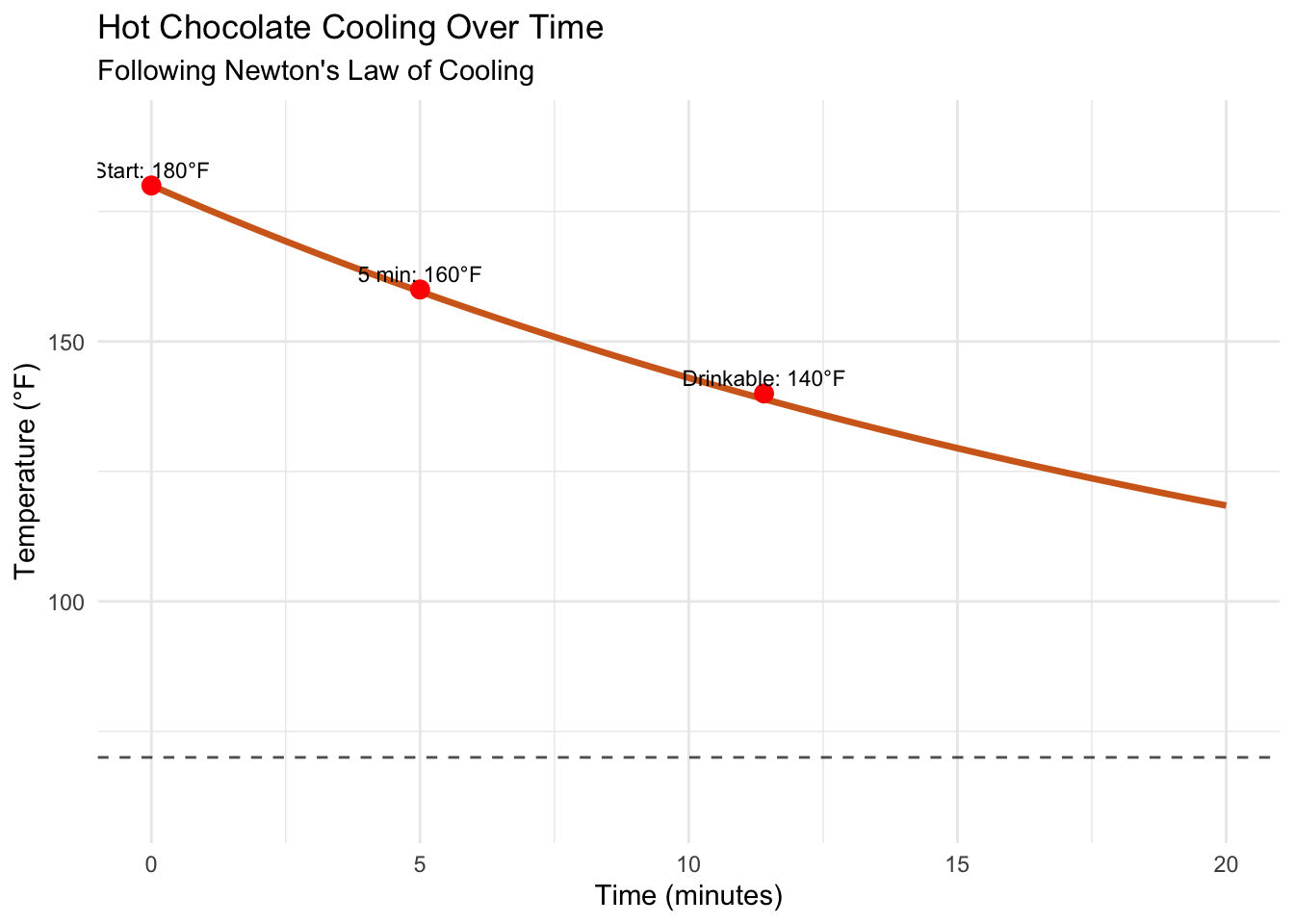
Notice the characteristic exponential decay curve. The temperature drops quickly at first when the difference between chocolate and room temperature is large, then slows as it approaches room temperature.
3.4 Beyond Simple Cooling: The Exponential Family
The technique we just used—separation of variables followed by integration—works for an entire family of differential equations. Any equation of the form:
\[\frac{dy}{dx} = ky\]
has the solution:
\[y(x) = y_0 e^{kx}\]
where \(y_0\) is the initial value at \(x = 0\).
This includes our population growth model from last time. Starting with:
\[\frac{dP}{dt} = rP\]
We separate variables:
\[\frac{dP}{P} = r , dt\]
Integrate both sides:
\[\ln|P| = rt + C\]
Exponentiate:
\[P(t) = P_0 e^{rt}\]
The same mathematical structure appears in radioactive decay (\(r\) negative), compound interest (discrete version), and bacterial growth (until resources become limited).
3.5 When Variables Refuse to Separate
Not every differential equation is separable, but many important ones are. Here’s a quick test: can you write the equation in the form \(\frac{dy}{dx} = g(x)h(y)\)? If yes, you can separate variables.
Consider the equation:
\[\frac{dy}{dx} = xy^2\]
This factors as \(\frac{dy}{dx} = x \cdot y^2\), so it’s separable. We can write:
\[\frac{dy}{y^2} = x , dx\]
Integrating both sides:
\[\int y^{-2} , dy = \int x , dx\] \[-\frac{1}{y} = \frac{x^2}{2} + C\]
Solving for \(y\):
\[y = -\frac{1}{\frac{x^2}{2} + C} = -\frac{2}{x^2 + 2C}\]
If we let \(K = 2C\), this becomes:
\[y = -\frac{2}{x^2 + K}\]
The value of \(K\) depends on initial conditions. If \(y(0) = -1\), then:
\[-1 = -\frac{2}{0 + K} = -\frac{2}{K}\]
So \(K = 2\), giving us:
\[y = -\frac{2}{x^2 + 2}\]
3.6 A More Complex Example: Mixing Problems
Imagine a 100-gallon tank initially filled with pure water. A brine solution containing 2 pounds of salt per gallon flows in at 3 gallons per minute, while the well-mixed solution flows out at the same rate. How much salt is in the tank after 20 minutes?
Let \(S(t)\) be the amount of salt (in pounds) at time \(t\). Salt enters at a rate of \(3 \text{ gal/min} \times 2 \text{ lb/gal} = 6 \text{ lb/min}\).
Salt leaves at a rate proportional to its concentration. Since the tank always contains 100 gallons, the concentration is \(\frac{S(t)}{100}\) lb/gal. With outflow at 3 gal/min, salt leaves at \(3 \times \frac{S(t)}{100} = \frac{3S(t)}{100}\) lb/min.
The differential equation becomes:
\[\frac{dS}{dt} = 6 - \frac{3S}{100}\]
This isn’t immediately separable because we can’t factor the right side as \(g(t)h(S)\). But we can rearrange:
\[\frac{dS}{dt} + \frac{3S}{100} = 6\]
Let’s substitute \(u = S - 200\) (we’ll see why in a moment). Then \(\frac{du}{dt} = \frac{dS}{dt}\), and since \(S = u + 200\):
\[\frac{du}{dt} + \frac{3(u + 200)}{100} = 6\] \[\frac{du}{dt} + \frac{3u}{100} + 6 = 6\] \[\frac{du}{dt} = -\frac{3u}{100}\]
This is separable! Following our standard procedure:
\[\frac{du}{u} = -\frac{3}{100} , dt\] \[\ln|u| = -\frac{3t}{100} + C\] \[u = A e^{-3t/100}\]
Since \(u = S - 200\):
\[S(t) = 200 + A e^{-3t/100}\]
With initial condition \(S(0) = 0\) (pure water initially):
\[0 = 200 + A\] \[A = -200\]
Therefore:
\[S(t) = 200(1 - e^{-3t/100})\]
After 20 minutes:
\[S(20) = 200(1 - e^{-3(20)/100}) = 200(1 - e^{-0.6}) \approx 200(1 - 0.549) \approx 90.2 \text{ pounds}\]
Let’s visualize this approach to equilibrium:
# Parameters for mixing problem
t <- seq(0, 100, by = 1)
S_t <- 200 * (1 - exp(-3*t/100))

# Create data frame
mixing_data <- data.frame(
  time = t,
  salt = S_t
)

# Plot the results
ggplot(mixing_data, aes(x = time, y = salt)) +
  geom_line(color = "steelblue", size = 1.2) +
  geom_hline(yintercept = 200, linetype = "dashed", alpha = 0.7) +
  geom_point(aes(x = 20, y = 200*(1-exp(-0.6))), color = "red", size = 3) +
  annotate("text", x = 25, y = 90, label = "20 min: 90.2 lbs", color = "red") +
  annotate("text", x = 70, y = 210, label = "Equilibrium: 200 lbs") +
  labs(
    title = "Salt Accumulation in Mixing Tank",
    x = "Time (minutes)",
    y = "Salt (pounds)",
    subtitle = "Approach to equilibrium concentration"
  ) +
  theme_minimal()
## Warning in geom_point(aes(x = 20, y = 200 * (1 - exp(-0.6))), color = "red", : All aesthetics have length 1, but the data has 101 rows.
## ℹ Please consider using `annotate()` or provide this layer with data containing a single row.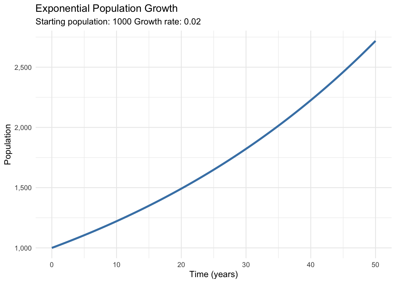
The curve shows salt content rising toward 200 pounds—the equilibrium where inflow and outflow balance. This S-shaped approach to equilibrium appears throughout physics, chemistry, and engineering.
3.7 The Power and Limits of Separation
Separation of variables works beautifully for equations where variables can be cleanly separated. But this method has limitations. Equations like:
\[\frac{dy}{dx} = x + y\]
or
\[\frac{dy}{dx} = \frac{x + y}{x - y}\]
can’t be solved by separation because their right sides don’t factor into \(g(x)h(y)\).
For such equations, we need other techniques—integrating factors, substitutions, or numerical methods. But separable equations form the foundation of differential equation solving because they’re both common and completely solvable with basic calculus.
3.8 Building Intuition
As you work with more differential equations, patterns emerge. Exponential functions arise naturally from equations where the rate of change is proportional to the current amount. Approaches to equilibrium often produce expressions like \(A(1 - e^{-kt})\). Oscillatory systems lead to trigonometric functions.
These aren’t just mathematical curiosities. They reflect deep truths about how natural systems behave. When you see \(e^{-kt}\) in a solution, you’re looking at a system approaching equilibrium. When you see \(e^{rt}\) with positive \(r\), you’re witnessing exponential growth that can’t continue indefinitely in the real world.
3.9 What’s Next
We’ve now mastered the art of solving separable differential equations—a surprisingly powerful technique that handles many real-world problems. But the differential equation landscape extends far beyond what separation of variables can reach.
In our next post, we’ll explore what happens when variables refuse to separate cleanly. We’ll learn about integrating factors, a technique that can tame certain linear equations, and we’ll discover when we need to abandon analytical solutions altogether in favor of numerical methods.
We’ll also start thinking about systems of differential equations—what happens when multiple quantities change simultaneously, each influencing the others. The interplay between predator and prey populations, the coupled oscillations of mechanical systems, and the feedback loops in economic models all require us to think beyond single equations.
The mathematical tools you’ve learned today—separation of variables, integration, and exponential solutions—form the bedrock for these more complex scenarios. Every system, no matter how complicated, can be understood by building up from these simple pieces.
The world may be complex, but it’s built from simple rules. We’re beginning to learn the language in which those rules are written.