Chapter 13 Average Reward in Reinforcement Learning: A Comprehensive Guide

The overwhelming majority of reinforcement learning (RL) literature centers on maximizing discounted cumulative rewards. This approach, while mathematically elegant and computationally convenient, represents just one way to formalize sequential decision-making problems. For many real-world applications—particularly those involving continuous operation without natural episode boundaries—an alternative formulation based on average reward per time step offers both theoretical advantages and practical benefits that deserve serious consideration.

13.1 The Limitations of Discounted Reward Formulations

Traditional RL formulates the control problem around maximizing the expected discounted return:

\[G_t = \sum_{k=0}^{\infty} \gamma^k R_{t+k+1}\]

where \(0 \leq \gamma < 1\) is the discount factor. The policy evaluation objective becomes:

\[J(\pi) = \mathbb{E}_\pi [G_t] = \mathbb{E}_\pi \left[ \sum_{k=0}^\infty \gamma^k R_{t+k+1} \right]\]

This formulation dominates the field for compelling mathematical reasons: it ensures convergence of infinite sums, provides contraction properties for Bellman operators, and offers computational tractability. However, these advantages come with conceptual costs that become apparent when we examine real-world applications.

Consider a server load balancing system that must operate continuously for months or years. In such systems, the choice of discount factor becomes arbitrary and potentially misleading. A discount factor of 0.9 implies that a reward received 22 steps in the future is worth only 10% of an immediate reward—a perspective that may not align with the true operational objectives. Similarly, in medical treatment scheduling, financial portfolio management, or industrial control systems, the fundamental goal is often to maximize long-term average performance rather than to optimize a present-value calculation with an artificially imposed time preference.

The prevalence of discounted formulations partly stems from RL’s historical focus on episodic tasks with clear terminal states. Games, navigation problems, and many benchmark environments naturally decompose into episodes with definite endings. However, this episodic perspective may be the exception rather than the rule in real-world applications. Manufacturing systems, recommendation engines, traffic control networks, and autonomous vehicles operate in continuing environments where the notion of “episodes” is artificial.

13.2 The Average Reward Alternative: Theoretical Foundations

The average reward formulation abandons discounting entirely, focusing instead on the long-run average payoff:

\[\rho(\pi) = \lim_{T \to \infty} \frac{1}{T} \; \mathbb{E}_\pi \left[ \sum_{t=1}^T R_t \right]\]

This quantity represents the steady-state reward rate under policy \(\pi\)—the expected reward per time step in the long run. The control problem becomes:

\[\pi^* = \arg\max_\pi \rho(\pi)\]

Unlike discounted formulations, this objective requires no arbitrary parameters and treats all time steps equally. The interpretation is straightforward: find the policy that maximizes long-term throughput.

The average reward formulation relies on ergodic theory for its theoretical foundation. Under standard assumptions—primarily that the Markov chains induced by policies are finite, irreducible, and aperiodic—several important properties hold. The well-definedness property ensures the limit defining \(\rho(\pi)\) exists and is finite. Initial state independence means the average reward is independent of the starting state. Finally, uniqueness of stationary distribution guarantees each policy induces a unique long-run state distribution.

These conditions are satisfied by most practical MDPs, making the average reward criterion broadly applicable. However, care must be taken with absorbing states or poorly connected state spaces, where ergodicity assumptions may fail.

A key insight is that average reward directly relates to the stationary distribution induced by a policy. If \(d^\pi(s)\) denotes the long-run probability of being in state \(s\) under policy \(\pi\), then:

\[\rho(\pi) = \sum_s d^\pi(s) \sum_a \pi(a|s) \sum_{s'} P(s'|s,a) R(s,a,s')\]

This expression reveals that optimizing average reward requires finding policies that induce favorable stationary distributions—those that concentrate probability mass on high-reward regions of the state space.

13.3 Value Functions in the Average Reward Setting

Without discounting, the traditional notion of value function becomes problematic. The infinite sum \(\sum_{k=0}^\infty R_{t+k+1}\) generally diverges, making it impossible to define meaningful state values in the conventional sense.

The solution is to work with relative values rather than absolute ones. The differential value function captures the relative advantage of starting in each state:

\[h_\pi(s) = \mathbb{E}_\pi \left[ \sum_{t=0}^\infty (R_{t+1} - \rho(\pi)) \;\big|\; S_0 = s \right]\]

This quantity measures how much better (or worse) it is to start in state \(s\) compared to the long-run average. Crucially, this sum converges under ergodic assumptions because the centered rewards \((R_{t+1} - \rho(\pi))\) have zero mean in the long run.

The differential value function satisfies a modified Bellman equation:

\[h_\pi(s) = \sum_a \pi(a|s) \sum_{s'} P(s'|s,a) \left[ R(s,a,s') - \rho(\pi) + h_\pi(s') \right]\]

This equation is structurally similar to the discounted case but with two key differences: the immediate reward is adjusted by subtracting the average reward, and no discount factor appears before the future differential value.

We can similarly define differential action-value functions:

\[q_\pi(s,a) = \sum_{s'} P(s'|s,a) \left[ R(s,a,s') - \rho(\pi) + h_\pi(s') \right]\]

These satisfy the consistency relation: \(h_\pi(s) = \sum_a \pi(a|s) q_\pi(s,a)\).

13.4 Optimality Theory for Average Reward

Optimal policies satisfy the average reward optimality equations:

\[\rho^* + h^*(s) = \max_a \sum_{s'} P(s'|s,a) \left[ R(s,a,s') + h^*(s') \right]\]

Here, \(\rho^*\) is the optimal average reward (achieved by any optimal policy), and \(h^*\) is the optimal differential value function. Unlike the discounted case, all optimal policies achieve the same average reward, though they may differ in their differential values.

The policy improvement theorem extends naturally to the average reward setting. Given the differential action-values under the current policy, improvement is achieved by acting greedily:

\[\pi'(s) = \arg\max_a q_\pi(s,a)\]

This greedy policy is guaranteed to achieve average reward \(\rho(\pi') \geq \rho(\pi)\), with equality only when \(\pi\) is already optimal.

13.5 Learning Algorithms for Average Reward

The most direct extension of TD learning to average reward settings involves updating both the differential value function and an estimate of the average reward. The average reward TD(0) algorithm proceeds as follows:

Initialize: \(h(s) = 0\) for all \(s\), \(\hat{\rho} = 0\)
For each time step \(t\):
- Observe \(S_t\), take action \(A_t\), observe \(R_{t+1}\) and \(S_{t+1}\)
- Compute TD error: \(\delta_t = R_{t+1} - \hat{\rho} + h(S_{t+1}) - h(S_t)\)
- Update differential value: \(h(S_t) \leftarrow h(S_t) + \alpha \delta_t\)
- Update average reward estimate: \(\hat{\rho} \leftarrow \hat{\rho} + \beta \delta_t\)

The step sizes \(\alpha\) and \(\beta\) control the learning rates for differential values and average reward, respectively. Typical choices satisfy \(\beta \ll \alpha\) to ensure the average reward estimate changes more slowly than differential values.

Convergence of average reward TD methods requires more delicate analysis than their discounted counterparts. The key challenge is that both \(h\) and \(\rho\) are being estimated simultaneously, creating a coupled system of stochastic approximations. Under standard assumptions (diminishing step sizes, sufficient exploration, ergodic Markov chains), convergence can be established using two-timescale analysis. The intuition is that \(\rho\) is estimated on a slower timescale (smaller step size), allowing the differential values to track the instantaneous policy while the average reward estimate provides a stable reference point.

Q-learning extends to average reward settings through the average reward Q-learning algorithm:

Initialize: \(q(s,a) = 0\) for all \((s,a)\), \(\hat{\rho} = 0\)
For each time step \(t\):
- Observe \(S_t\), choose \(A_t\) (e.g., \(\epsilon\)-greedily)
- Observe \(R_{t+1}\) and \(S_{t+1}\)
- Compute TD error: \(\delta_t = R_{t+1} - \hat{\rho} + \max_a q(S_{t+1}, a) - q(S_t, A_t)\)
- Update: \(q(S_t, A_t) \leftarrow q(S_t, A_t) + \alpha \delta_t\)
- Update: \(\hat{\rho} \leftarrow \hat{\rho} + \beta \delta_t\)

This algorithm learns differential action-values directly, avoiding the need to maintain a separate state value function.

13.6 Practical Implementation: Server Load Balancing

Consider a web server load balancing system with three servers. Requests arrive continuously and must be routed to minimize average response time. This is naturally a continuing task where episodes don’t exist, making it ideal for average reward formulation.

# Server Load Balancing with Average Reward Q-Learning
library(ggplot2)

# Environment setup
set.seed(42)
n_servers <- 3
max_load <- 5
n_steps <- 50000

# State encoding and reward function
encode_state <- function(loads) {
  sum(loads * (max_load + 1)^(0:(length(loads)-1))) + 1
}

decode_state <- function(state_id) {
  state_id <- state_id - 1
  loads <- numeric(n_servers)
  for (i in 1:n_servers) {
    loads[i] <- state_id %% (max_load + 1)
    state_id <- state_id %/% (max_load + 1)
  }
  loads
}

get_reward <- function(loads, server_choice) {
  new_loads <- loads
  new_loads[server_choice] <- min(new_loads[server_choice] + 1, max_load)
  
  # Response time model: linear in load
  avg_load <- mean(new_loads)
  reward <- -avg_load
  
  # Simulate request completion
  for (i in 1:n_servers) {
    if (new_loads[i] > 0 && runif(1) < 0.3) {
      new_loads[i] <- new_loads[i] - 1
    }
  }
  
  list(reward = reward, new_loads = new_loads)
}

# Initialize parameters
n_states <- (max_load + 1)^n_servers
Q <- array(0, dim = c(n_states, n_servers))
rho_hat <- 0
alpha <- 0.1
beta <- 0.001
epsilon <- 0.1

# Training loop
loads <- rep(0, n_servers)
state_id <- encode_state(loads)
rewards_history <- numeric(n_steps)
rho_history <- numeric(n_steps)

cat("Training average reward Q-learning agent...\n")

## Training average reward Q-learning agent...

for (step in 1:n_steps) {
  # Epsilon-greedy action selection
  if (runif(1) < epsilon) {
    action <- sample(1:n_servers, 1)
  } else {
    action <- which.max(Q[state_id, ])
  }
  
  # Take action and observe reward
  result <- get_reward(loads, action)
  reward <- result$reward
  loads <- result$new_loads
  next_state_id <- encode_state(loads)
  
  # Q-learning update
  td_error <- reward - rho_hat + max(Q[next_state_id, ]) - Q[state_id, action]
  Q[state_id, action] <- Q[state_id, action] + alpha * td_error
  rho_hat <- rho_hat + beta * td_error
  
  # Record progress
  rewards_history[step] <- reward
  rho_history[step] <- rho_hat
  
  # Update state
  state_id <- next_state_id
  
  # Decay exploration
  if (step %% 1000 == 0) {
    epsilon <- max(0.01, epsilon * 0.995)
    if (step %% 10000 == 0) {
      cat(sprintf("Step %d: Average reward estimate = %.4f\n", step, rho_hat))
    }
  }
}

## Step 10000: Average reward estimate = -1.5199
## Step 20000: Average reward estimate = -1.6557
## Step 30000: Average reward estimate = -1.6660
## Step 40000: Average reward estimate = -1.6685
## Step 50000: Average reward estimate = -1.6553

# Evaluate learned policy
eval_steps <- 10000
loads <- rep(0, n_servers)
state_id <- encode_state(loads)
eval_rewards <- numeric(eval_steps)

for (step in 1:eval_steps) {
  action <- which.max(Q[state_id, ])
  result <- get_reward(loads, action)
  eval_rewards[step] <- result$reward
  loads <- result$new_loads
  state_id <- encode_state(loads)
}

final_avg_reward <- mean(eval_rewards)
cat(sprintf("Final average reward: %.4f\n", final_avg_reward))

## Final average reward: -1.6658

cat(sprintf("Training estimate: %.4f\n", rho_hat))

## Training estimate: -1.6553

# Policy analysis
cat("\nLearned policy examples:\n")

## 
## Learned policy examples:

example_states <- list(
  c(0, 0, 0),  # All servers idle
  c(3, 1, 1),  # Server 1 heavily loaded
  c(2, 2, 2),  # Balanced load
  c(5, 0, 0),  # Server 1 at capacity
  c(3, 3, 4)   # High overall load
)

for (i in seq_along(example_states)) {
  loads <- example_states[[i]]
  state_id <- encode_state(loads)
  q_values <- Q[state_id, ]
  best_action <- which.max(q_values)
  
  cat(sprintf("Loads %s -> Route to server %d (Q-values: %.3f, %.3f, %.3f)\n",
              paste(loads, collapse=", "), best_action,
              q_values[1], q_values[2], q_values[3]))
}

## Loads 0, 0, 0 -> Route to server 2 (Q-values: -0.033, 0.000, 0.000)
## Loads 3, 1, 1 -> Route to server 3 (Q-values: -0.249, -0.171, -0.116)
## Loads 2, 2, 2 -> Route to server 2 (Q-values: -0.434, -0.355, -0.408)
## Loads 5, 0, 0 -> Route to server 3 (Q-values: -0.166, -0.214, -0.154)
## Loads 3, 3, 4 -> Route to server 1 (Q-values: -0.884, -1.003, -0.918)

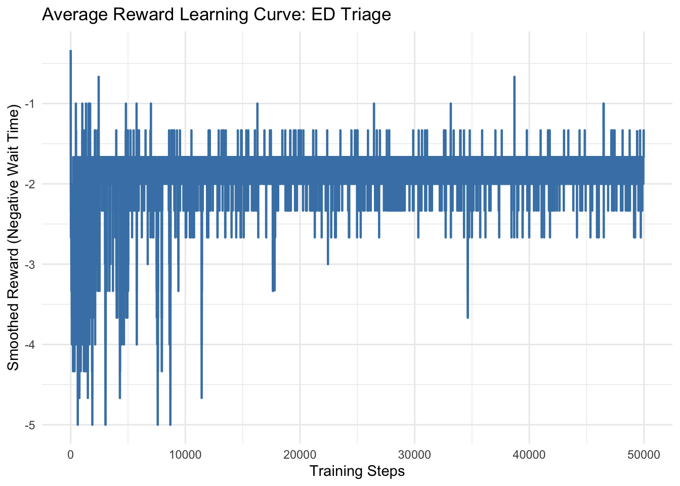
13.7 Implementation Considerations

The choice of step sizes \(\alpha\) and \(\beta\) is crucial for average reward algorithms. The general principle is to use different timescales: a fast timescale (\(\alpha\)) for updates to value functions or policy parameters, and a slow timescale (\(\beta\)) for updates to the average reward estimate. A common choice is \(\beta = c \cdot \alpha\) where \(c \in [0.01, 0.1]\). This ensures the average reward estimate stabilizes while allowing value functions to adapt to policy changes.

Unlike discounted RL, where initialization typically has limited impact on final performance, average reward methods can be sensitive to initial conditions. Poor initialization of \(\hat{\rho}\) can lead to slow convergence or temporary instability. Effective strategies include running a random policy for some steps to get an initial estimate of \(\hat{\rho}\), starting with a conservative estimate based on domain knowledge, or using adaptive step sizes that are larger initially and then decay as estimates stabilize.

Exploration-exploitation trade-offs require special consideration in average reward settings. Since there’s no discounting to naturally prioritize immediate rewards, exploration strategies must be designed to maintain long-term effectiveness. Optimistic initialization works particularly well: initializing value functions optimistically encourages exploration while the agent discovers the true reward structure.

13.8 When to Choose Average Reward Over Discounting

The choice between discounted and average reward formulations should be based on problem characteristics rather than mathematical convenience. Consider average reward when the task is genuinely continuing with no natural episodes, long-term steady-state performance is the primary concern, the discount factor feels arbitrary or its choice significantly affects learned behavior, or fairness across time steps is important.

Moderate indicators include when the environment is relatively stable over long horizons, exploration can be maintained without artificial urgency from discounting, or the system will operate for extended periods without reset. However, choose against average reward when the task has clear episodes or terminal states, short-term performance is crucial (e.g., real-time systems), the environment is highly non-stationary, or mathematical tractability is paramount.

Based on empirical studies and practical applications, server systems and manufacturing typically find average reward superior, while games with clear episodes often find discounting more natural. Financial trading uses average reward for long-term strategies and discounting for short-term tactics. In robotics, the choice depends on task duration and safety requirements, while recommendation systems use average reward for user satisfaction and discounting for engagement.

13.9 Appendix A: Mathematical Proofs and Derivations

13.9.1 Convergence of Average Reward TD Learning

Theorem: Under standard assumptions (finite state space, ergodic Markov chains, diminishing step sizes satisfying \(\sum_t \alpha_t = \infty\), \(\sum_t \alpha_t^2 < \infty\), and \(\beta_t = o(\alpha_t)\)), the average reward TD(0) algorithm converges almost surely to the true differential value function and average reward.

Proof sketch: The proof uses two-timescale stochastic approximation theory. The key insight is that the average reward estimate evolves on a slower timescale (smaller step size), allowing it to track the average while the differential values adapt to the current estimate.

Let \(\{\alpha_t\}\) and \(\{\beta_t\}\) be the step size sequences for differential values and average reward, respectively, satisfying \(\beta_t = o(\alpha_t)\).

The updates can be written as: \[h_{t+1}(s) = h_t(s) + \alpha_t \mathbf{1}_{S_t = s} [R_{t+1} - \rho_t + h_t(S_{t+1}) - h_t(S_t)]\] \[\rho_{t+1} = \rho_t + \beta_t [R_{t+1} - \rho_t + h_t(S_{t+1}) - h_t(S_t)]\]

Using the two-timescale framework, we first analyze the faster timescale (differential values) assuming the average reward estimate is fixed. This leads to the standard convergence analysis for policy evaluation. Then, we analyze the slower timescale (average reward) and show it tracks the true average reward under the converged policy.

13.9.2 Policy Gradient Theorem for Average Reward

Theorem (Average Reward Policy Gradient): For a parameterized policy \(\pi_\theta\), the gradient of the average reward with respect to parameters is:

\[\nabla_\theta \rho(\pi_\theta) = \sum_s d^{\pi_\theta}(s) \sum_a \nabla_\theta \pi_\theta(a|s) q^{\pi_\theta}(s,a)\]

where \(d^{\pi_\theta}(s)\) is the stationary distribution under policy \(\pi_\theta\) and \(q^{\pi_\theta}(s,a)\) is the differential action-value function.

Proof: The proof parallels the discounted case but requires careful handling of the limit defining average reward. The key steps involve expressing average reward in terms of stationary distribution, differentiating with respect to \(\theta\), applying the chain rule noting that both the stationary distribution and immediate rewards depend on the policy, using the fundamental matrix approach to handle the derivative of the stationary distribution, and simplifying using the relationship between immediate rewards and differential action-values.

13.9.3 Optimality Equations Derivation

Starting from the definition of differential value function: \[h^*(s) = \max_\pi h^\pi(s)\]

where \[h^\pi(s) = \mathbb{E}^\pi \left[ \sum_{t=0}^\infty (R_{t+1} - \rho(\pi)) \mid S_0 = s \right]\]

For the optimal policy \(\pi^*\), we have: \[h^*(s) = \mathbb{E}^{\pi^*} \left[ \sum_{t=0}^\infty (R_{t+1} - \rho^*) \mid S_0 = s \right]\]

Expanding the first term and using the Markov property, since \(\pi^*\) is optimal, it must choose actions to maximize: \[\sum_{s'} P(s'|s,a) [R(s,a,s') - \rho^* + h^*(s')]\]

This gives us the optimality equation: \[\rho^* + h^*(s) = \max_a \sum_{s'} P(s'|s,a) [R(s,a,s') + h^*(s')]\]

The average reward formulation of reinforcement learning provides a principled alternative to discounted approaches that better captures the objectives of many real-world applications. While mathematically more challenging than discounted methods, the conceptual clarity and practical benefits make it worthy of broader adoption. The choice between formulations should reflect true problem objectives rather than mathematical convenience, and for many continuing tasks, average reward optimization represents the most appropriate objective for creating systems that serve genuine long-term value.