Chapter 9 Dyna and DynaQ
9.1 Introduction
Traditional reinforcement learning methods fall into two categories: model-free approaches like SARSA and Q-Learning that learn directly from experience, and model-based methods that first learn environment dynamics then use planning algorithms. Dyna, introduced by Sutton (1990), bridges this gap by combining direct reinforcement learning with indirect learning through an internal model of the environment.
The key insight behind Dyna is that real experience can serve dual purposes: updating value functions directly and improving an internal model that generates simulated experience for additional learning. This architecture allows agents to benefit from both the sample efficiency of planning and the robustness of direct learning, making it particularly effective in environments where experience is costly or limited.
9.2 Theoretical Framework
9.2.1 The Dyna Architecture
Dyna integrates three key components within a unified learning system:
- Direct RL: Learning from real experience using standard temporal difference methods
- Model Learning: Building an internal model of environment dynamics from experience
- Planning: Using the learned model to generate simulated experience for additional value function updates
The complete Dyna update cycle can be formalized as follows. For each real experience tuple \((s, a, r, s')\):
Direct Learning (Q-Learning): \[Q(s,a) \leftarrow Q(s,a) + \alpha \left[ r + \gamma \max_{a'} Q(s', a') - Q(s,a) \right]\]
Model Update: \[\hat{T}(s,a) \leftarrow s'\] \[\hat{R}(s,a) \leftarrow r\]
Planning Phase (repeat \(n\) times): \[s \leftarrow \text{random previously visited state}\] \[a \leftarrow \text{random action previously taken in } s\] \[r \leftarrow \hat{R}(s,a)\] \[s' \leftarrow \hat{T}(s,a)\] \[Q(s,a) \leftarrow Q(s,a) + \alpha \left[ r + \gamma \max_{a'} Q(s', a') - Q(s,a) \right]\]
The parameter \(n\) controls the number of planning steps per real experience, representing the computational budget available for internal simulation.
9.2.2 Model Representation
In its simplest form, Dyna uses a deterministic table-based model where \(\hat{T}(s,a)\) stores the last observed next state for state-action pair \((s,a)\), and \(\hat{R}(s,a)\) stores the last observed reward. This approach works well for deterministic environments but can be extended to handle stochastic dynamics through sampling-based representations.
9.2.3 Convergence Properties
Under standard assumptions (all state-action pairs visited infinitely often, appropriate learning rates), Dyna inherits the convergence guarantees of its underlying RL algorithm. The addition of planning typically accelerates convergence by allowing each real experience to propagate information more widely through the value function.
9.3 Implementation in R
We implement Dyna-Q using the same 10-state environment from previous posts, allowing direct comparison with pure Q-Learning and SARSA approaches.
9.3.1 Environment Setup
# Environment parameters
n_states <- 10
n_actions <- 2
gamma <- 0.9
terminal_state <- n_states

# Transition and reward models (same as previous posts)
set.seed(42)
transition_model <- array(0, dim = c(n_states, n_actions, n_states))
reward_model <- array(0, dim = c(n_states, n_actions, n_states))

for (s in 1:(n_states - 1)) {
  transition_model[s, 1, s + 1] <- 0.9
  transition_model[s, 1, sample(1:n_states, 1)] <- 0.1
  transition_model[s, 2, sample(1:n_states, 1)] <- 0.8
  transition_model[s, 2, sample(1:n_states, 1)] <- 0.2

  for (s_prime in 1:n_states) {
    reward_model[s, 1, s_prime] <- ifelse(s_prime == n_states, 1.0, 0.1 * runif(1))
    reward_model[s, 2, s_prime] <- ifelse(s_prime == n_states, 0.5, 0.05 * runif(1))
  }
}

transition_model[n_states, , ] <- 0
reward_model[n_states, , ] <- 0

# Environment interaction function
sample_env <- function(s, a) {
  probs <- transition_model[s, a, ]
  s_prime <- sample(1:n_states, 1, prob = probs)
  reward <- reward_model[s, a, s_prime]
  list(s_prime = s_prime, reward = reward)
}
9.3.2 Dyna-Q Implementation
# Dyna-Q algorithm with episode-wise performance tracking
dyna_q <- function(episodes = 1000, alpha = 0.1, epsilon = 0.1, n_planning = 5) {
  Q <- matrix(0, nrow = n_states, ncol = n_actions)
  model_T <- array(NA, dim = c(n_states, n_actions))
  model_R <- array(NA, dim = c(n_states, n_actions))
  visited_sa <- list()

  episode_rewards <- numeric(episodes)
  episode_steps <- numeric(episodes)

  for (ep in 1:episodes) {
    s <- 1
    total_reward <- 0
    steps <- 0

    while (s != terminal_state && steps < 100) {  # Add max steps to prevent infinite loops
      if (runif(1) < epsilon) {
        a <- sample(1:n_actions, 1)
      } else {
        a <- which.max(Q[s, ])
      }

      outcome <- sample_env(s, a)
      s_prime <- outcome$s_prime
      r <- outcome$reward

      total_reward <- total_reward + r
      steps <- steps + 1

      Q[s, a] <- Q[s, a] + alpha * (r + gamma * max(Q[s_prime, ]) - Q[s, a])

      model_T[s, a] <- s_prime
      model_R[s, a] <- r

      sa_key <- paste(s, a, sep = "_")
      if (!(sa_key %in% names(visited_sa))) {
        visited_sa[[sa_key]] <- c(s, a)
      }

      if (length(visited_sa) > 0) {
        for (i in 1:n_planning) {
          sa_sample <- sample(visited_sa, 1)[[1]]
          s_plan <- sa_sample[1]
          a_plan <- sa_sample[2]

          if (!is.na(model_T[s_plan, a_plan])) {
            s_prime_plan <- model_T[s_plan, a_plan]
            r_plan <- model_R[s_plan, a_plan]

            Q[s_plan, a_plan] <- Q[s_plan, a_plan] +
              alpha * (r_plan + gamma * max(Q[s_prime_plan, ]) - Q[s_plan, a_plan])
          }
        }
      }

      s <- s_prime
    }

    episode_rewards[ep] <- total_reward
    episode_steps[ep] <- steps
  }

  list(Q = Q, policy = apply(Q, 1, which.max),
       episode_rewards = episode_rewards, episode_steps = episode_steps)
}

# Q-Learning with performance tracking
q_learning <- function(episodes = 1000, alpha = 0.1, epsilon = 0.1) {
  Q <- matrix(0, nrow = n_states, ncol = n_actions)
  episode_rewards <- numeric(episodes)
  episode_steps <- numeric(episodes)

  for (ep in 1:episodes) {
    s <- 1
    total_reward <- 0
    steps <- 0

    while (s != terminal_state && steps < 100) {
      a <- if (runif(1) < epsilon) sample(1:n_actions, 1) else which.max(Q[s, ])
      outcome <- sample_env(s, a)
      s_prime <- outcome$s_prime
      r <- outcome$reward

      total_reward <- total_reward + r
      steps <- steps + 1

      Q[s, a] <- Q[s, a] + alpha * (r + gamma * max(Q[s_prime, ]) - Q[s, a])
      s <- s_prime
    }

    episode_rewards[ep] <- total_reward
    episode_steps[ep] <- steps
  }

  list(Q = Q, policy = apply(Q, 1, which.max),
       episode_rewards = episode_rewards, episode_steps = episode_steps)
}
9.4 Experimental Analysis
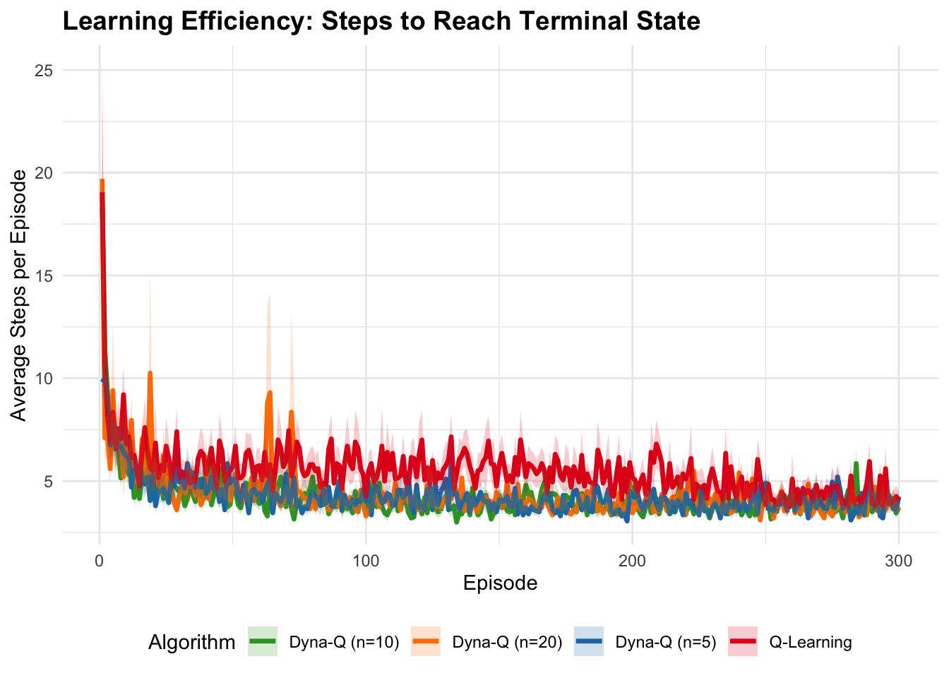
9.4.1 Learning Efficiency Comparison
We compare Dyna-Q against standard Q-Learning across different numbers of planning steps:
# Run comprehensive experiments
set.seed(123)
n_runs <- 20
episodes <- 300

# Initialize results storage
all_results <- data.frame()

print("Running experiments...")
## [1] "Running experiments..."for (run in 1:n_runs) {
cat("Run", run, "of", n_runs, "\n")
# Run algorithms
ql_result <- q_learning(episodes = episodes)
dyna5_result <- dyna_q(episodes = episodes, n_planning = 5)
dyna10_result <- dyna_q(episodes = episodes, n_planning = 10)
dyna20_result <- dyna_q(episodes = episodes, n_planning = 20)
# Store results
run_data <- data.frame(
episode = rep(1:episodes, 4),
run = run,
algorithm = rep(c("Q-Learning", "Dyna-Q (n=5)", "Dyna-Q (n=10)", "Dyna-Q (n=20)"), each = episodes),
reward = c(ql_result$episode_rewards, dyna5_result$episode_rewards,
dyna10_result$episode_rewards, dyna20_result$episode_rewards),
steps = c(ql_result$episode_steps, dyna5_result$episode_steps,
dyna10_result$episode_steps, dyna20_result$episode_steps)
)
all_results <- rbind(all_results, run_data)
}## Run 1 of 20
## Run 2 of 20
## Run 3 of 20
## Run 4 of 20
## Run 5 of 20
## Run 6 of 20
## Run 7 of 20
## Run 8 of 20
## Run 9 of 20
## Run 10 of 20
## Run 11 of 20
## Run 12 of 20
## Run 13 of 20
## Run 14 of 20
## Run 15 of 20
## Run 16 of 20
## Run 17 of 20
## Run 18 of 20
## Run 19 of 20
## Run 20 of 20##
## Attaching package: 'dplyr'## The following object is masked from 'package:gridExtra':
##
## combine## The following objects are masked from 'package:stats':
##
## filter, lag## The following objects are masked from 'package:base':
##
## intersect, setdiff, setequal, unionlibrary(ggplot2)
# Compute smoothed averages
smoothed_results <- all_results %>%
group_by(algorithm, episode) %>%
summarise(
mean_reward = mean(reward),
se_reward = sd(reward) / sqrt(n()),
mean_steps = mean(steps),
se_steps = sd(steps) / sqrt(n()),
.groups = 'drop'
) %>%
group_by(algorithm) %>%
mutate(
smooth_reward = stats::filter(mean_reward, rep(1/10, 10), sides = 2),
smooth_steps = stats::filter(mean_steps, rep(1/10, 10), sides = 2)
)
# Create comprehensive visualization
# Plot 1: Learning Curves (Rewards)
p1 <- ggplot(smoothed_results, aes(x = episode, y = mean_reward, color = algorithm)) +
geom_line(size = 1.2) +
geom_ribbon(aes(ymin = mean_reward - se_reward, ymax = mean_reward + se_reward, fill = algorithm),
alpha = 0.2, color = NA) +
scale_color_manual(values = c("Q-Learning" = "#E31A1C", "Dyna-Q (n=5)" = "#1F78B4",
"Dyna-Q (n=10)" = "#33A02C", "Dyna-Q (n=20)" = "#FF7F00")) +
scale_fill_manual(values = c("Q-Learning" = "#E31A1C", "Dyna-Q (n=5)" = "#1F78B4",
"Dyna-Q (n=10)" = "#33A02C", "Dyna-Q (n=20)" = "#FF7F00")) +
labs(title = "Learning Performance: Average Episode Rewards",
x = "Episode", y = "Average Reward per Episode",
color = "Algorithm", fill = "Algorithm") +
theme_minimal() +
theme(plot.title = element_text(size = 14, face = "bold"),
legend.position = "bottom")## Warning: Using `size` aesthetic for lines was deprecated in ggplot2 3.4.0.
## ℹ Please use `linewidth` instead.
## This warning is displayed once every 8 hours.
## Call `lifecycle::last_lifecycle_warnings()` to see where this warning was generated.# Plot 2: Steps to Terminal (Efficiency)
p2 <- ggplot(smoothed_results, aes(x = episode, y = mean_steps, color = algorithm)) +
geom_line(size = 1.2) +
geom_ribbon(aes(ymin = mean_steps - se_steps, ymax = mean_steps + se_steps, fill = algorithm),
alpha = 0.2, color = NA) +
scale_color_manual(values = c("Q-Learning" = "#E31A1C", "Dyna-Q (n=5)" = "#1F78B4",
"Dyna-Q (n=10)" = "#33A02C", "Dyna-Q (n=20)" = "#FF7F00")) +
scale_fill_manual(values = c("Q-Learning" = "#E31A1C", "Dyna-Q (n=5)" = "#1F78B4",
"Dyna-Q (n=10)" = "#33A02C", "Dyna-Q (n=20)" = "#FF7F00")) +
labs(title = "Learning Efficiency: Steps to Reach Terminal State",
x = "Episode", y = "Average Steps per Episode",
color = "Algorithm", fill = "Algorithm") +
theme_minimal() +
theme(plot.title = element_text(size = 14, face = "bold"),
legend.position = "bottom")
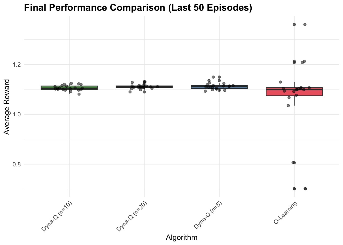
# Plot 3: Final performance comparison (last 50 episodes)
final_performance <- all_results %>%
filter(episode > episodes - 50) %>%
group_by(algorithm, run) %>%
summarise(avg_reward = mean(reward), .groups = 'drop')
p3 <- ggplot(final_performance, aes(x = algorithm, y = avg_reward, fill = algorithm)) +
geom_boxplot(alpha = 0.7) +
geom_point(position = position_jitter(width = 0.2), alpha = 0.5) +
scale_fill_manual(values = c("Q-Learning" = "#E31A1C", "Dyna-Q (n=5)" = "#1F78B4",
"Dyna-Q (n=10)" = "#33A02C", "Dyna-Q (n=20)" = "#FF7F00")) +
labs(title = "Final Performance Comparison (Last 50 Episodes)",
x = "Algorithm", y = "Average Reward",
fill = "Algorithm") +
theme_minimal() +
theme(plot.title = element_text(size = 14, face = "bold"),
axis.text.x = element_text(angle = 45, hjust = 1),
legend.position = "none")
# Display all plots
print(p1)
9.5 Discussion
Dyna demonstrates a fundamental trade-off between sample efficiency and computational cost, requiring \((n+1)\) times the computation per step compared to model-free methods due to additional planning updates. This computational investment typically yields faster convergence, particularly when real experience is expensive or dangerous to obtain, though optimal planning steps depend on problem characteristics—moderate values (5-10) generally provide good improvements without excessive overhead while very large values can produce diminishing returns or hurt performance with inaccurate models. The algorithm’s effectiveness critically depends on model quality, with our deterministic table-based implementation becoming increasingly accurate as more state-action pairs are visited, though this approach assumes deterministic transitions and uses simple model representation (storing only last observed transitions) that works well for stationary environments but struggles with non-stationary dynamics where more sophisticated representations maintaining transition probability distributions could improve robustness at increased computational cost. The interaction between exploration and planning creates a distinctive advantage where \(\epsilon\)-greedy exploration ensures diverse state-action coverage that directly improves model quality and planning effectiveness, establishing a positive feedback loop where better exploration enhances the model, making planning more effective and leading to better policies with potentially more informed exploration. Relative to pure model-free methods like Q-Learning, Dyna typically shows faster convergence and better sample efficiency by allowing each real experience to propagate information more widely through planning, while compared to pure model-based approaches, it maintains robustness through continued direct learning even with imperfect models. However, basic Dyna has notable limitations including poor representation of stochastic environments through deterministic models and suboptimal uniform sampling for planning, though modern extensions like Dyna-Q+ with exploration bonuses, prioritized sweeping focusing on high-value updates, and model-based variants maintaining probability distributions over transitions address many of these constraints.
9.6 Implementation Considerations and Conclusion
Dyna requires additional memory to store the learned model alongside the value function. In our implementation, this doubles the memory requirements compared to pure Q-Learning. For larger state-action spaces, this can become a significant consideration, potentially requiring sparse representations or function approximation techniques. The planning phase introduces variable computational demands that can complicate real-time applications. While the number of planning steps can be adjusted based on available computational budget, this flexibility requires careful consideration of timing constraints in online learning scenarios. Dyna introduces additional hyperparameters, particularly the number of planning steps \(n\). This parameter requires tuning based on the specific problem characteristics and computational constraints. Unlike some hyperparameters that can be set based on theoretical considerations, \(n\) often requires empirical validation.
Dyna represents an elegant solution to integrating learning and planning in reinforcement learning, combining the sample efficiency of model-based methods with the robustness of model-free approaches. Our R implementation demonstrates both the benefits and challenges of this integration, showing improved learning speed at the cost of increased computational and memory requirements. The key insight of using real experience for both direct learning and model improvement creates a powerful synergy that can significantly accelerate learning in many environments. However, the approach requires careful consideration of model representation, computational constraints, and hyperparameter tuning to achieve optimal performance. Future extensions could explore more sophisticated model representations, prioritized planning strategies, or integration with function approximation techniques for handling larger state spaces. The fundamental principle of combining direct and indirect learning remains a valuable paradigm in modern reinforcement learning research.