Chapter 14 Eligibility Traces

14.1 From One-Step to Multi-Step Learning

The preceding discussion on average reward reinforcement learning focused on algorithms like TD(0) and Q-learning, which update value estimates based on a one-step lookahead. These methods, known as one-step temporal-difference (TD) methods, perform a “bootstrap” from the value of the very next state. While computationally efficient, this approach can be slow to propagate information through the state space. An error discovered in one state only trickles back to its predecessor on the next visit. For tasks with long causal chains between actions and significant rewards, this one-step credit assignment process becomes a bottleneck, leading to slow convergence.

Eligibility traces offer a powerful and elegant mechanism to address this limitation. They provide a bridge between one-step TD methods and computationally expensive Monte Carlo (MC) methods, which update state values only at the end of an episode based on the full sequence of rewards. By maintaining a memory of recently visited states, eligibility traces allow a single TD error to be used to update the values of multiple preceding states simultaneously, dramatically accelerating the learning process. This follow-up explores the theory and application of eligibility traces, with a particular focus on their integration into the average reward framework.

14.2 The Mechanics of Eligibility Traces: A Backward View

At its core, an eligibility trace is a short-term memory vector, denoted \(e\_t \\in \\mathbb{R}^{|\\mathcal{S}|}\) for state-value functions or \(e\_t \\in \\mathbb{R}^{|\\mathcal{S}| \\times |\\mathcal{A}|}\) for action-value functions. Each component of this vector corresponds to a state (or state-action pair) and records a measure of its “eligibility” for learning from the current TD error. A state’s eligibility is highest immediately after it is visited and then decays exponentially over time.

The most common form of trace is the accumulating trace. At each time step \(t\), the trace for the current state \(S\_t\) is incremented, while the traces for all other states decay. The update rule is given by:

\[e_t(s) = \begin{cases} \lambda e_{t-1}(s) + 1 & \text{if } s = S_t \\ \lambda e_{t-1}(s) & \text{if } s \neq S_t \end{cases}\]

for all \(s \\in \\mathcal{S}\). The parameter \(\\lambda \\in [0, 1]\) is the trace-decay parameter. It controls the rate at which the trace fades. When \(\\lambda = 0\), the trace vector is non-zero only for the current state, \(e\_t(S\_t)=1\), which reduces the algorithm to a one-step TD method. As \(\\lambda\) approaches 1, the traces of past states decay more slowly, and credit from a TD error is assigned more broadly to states visited further in the past. When \(\\lambda=1\), the update becomes closely related to Monte Carlo methods, where credit is distributed across all prior states in an episode.

This formulation is known as the backward view of learning with eligibility traces. The term “backward” refers to the mechanism: at time \(t+1\), the TD error \(\\delta\_t\) is computed and then used to update the value estimates of states visited before time \(t\), with the magnitude of the update for each state weighted by its current trace value.

14.3 The TD(\(\\lambda\)) Algorithm for Prediction

The canonical prediction algorithm using eligibility traces is TD(\(\\lambda\)). It combines the trace mechanism with the standard TD update. For policy evaluation in the average reward setting, the goal is to learn the differential value function \(h\_\\pi(s)\). The algorithm proceeds as follows:

Initialize \(h(s)\) for all \(s \\in \\mathcal{S}\), and the average reward estimate \(\\hat{\\rho}\).
Initialize the eligibility trace vector \(e(s) = 0\) for all \(s\).
For each time step \(t\):
1. Observe state \(S\_t\), take action \(A\_t\) (according to policy \(\\pi\)), and observe reward \(R\_{t+1}\) and next state \(S\_{t+1}\).
2. Compute the differential TD error: \[\delta_t = R_{t+1} - \hat{\rho} + h(S_{t+1}) - h(S_t)\]
3. Decay all traces and increment the trace for the current state: \[e(s) \leftarrow \lambda e(s) \text{ for all } s \in \mathcal{S}\] \[e(S_t) \leftarrow e(S_t) + 1\]
4. Update the value function and average reward estimate for all states: \[h(s) \leftarrow h(s) + \alpha \delta_t e(s) \text{ for all } s \in \mathcal{S}\] \[\hat{\rho} \leftarrow \hat{\rho} + \beta \delta_t\]

The crucial difference from the one-step TD(0) algorithm lies in step 3d. Instead of updating only the value of the current state \(S\_t\), TD(\(\\lambda\)) updates the value of every state in proportion to its eligibility trace. A state visited many time steps ago, but whose trace has not fully decayed, will still receive a portion of the learning update from the current TD error. This allows a single surprising outcome (a large \(\\delta\_t\)) to immediately inform the values of all states in the causal chain leading up to it.

The theoretical justification for this backward mechanism comes from the forward view, which defines a compound target called the \(\\lambda\)-return. The \(\\lambda\)-return \(G\_t^\\lambda\) is an exponentially weighted average of n-step returns. In the average reward setting, the n-step differential return is:

\[G_{t:t+n} = \sum_{k=0}^{n-1} (R_{t+k+1} - \hat{\rho}) + h(S_{t+n})\]

The TD(\(\\lambda\)) update, as implemented via the backward view with eligibility traces, has been shown to be an efficient and unbiased way to approximate an update toward the \(\\lambda\)-return, making it a sound and powerful learning rule.

14.4 Control with Eligibility Traces: Average Reward Sarsa(\(\\lambda\))

Extending eligibility traces from prediction to control requires applying them to action-value functions. The most direct on-policy control algorithm is Sarsa(\(\\lambda\)). It follows the same principles as TD(\(\\lambda\)) but learns a differential action-value function \(q(s,a)\) instead of a state-value function \(h(s)\). The name Sarsa derives from the quintuple of events that form the basis of its update: \((S\_t, A\_t, R\_{t+1}, S\_{t+1}, A\_{t+1})\).

In the average reward context, the Sarsa(\(\\lambda\)) algorithm maintains an eligibility trace for each state-action pair, \(e(s,a)\). The update proceeds as follows:

Initialize \(q(s,a)\) for all \((s,a)\), and the average reward estimate \(\\hat{\\rho}\).
Initialize the eligibility trace vector \(e(s,a) = 0\) for all \((s,a)\).
Choose an initial state \(S\_0\) and an initial action \(A\_0\) (e.g., \(\\epsilon\)-greedily from \(q(S\_0, \\cdot)\)).
For each time step \(t\):
1. Take action \(A\_t\), observe reward \(R\_{t+1}\) and next state \(S\_{t+1}\).
2. Choose the next action \(A\_{t+1}\) from \(S\_{t+1}\) using the policy derived from \(q\) (e.g., \(\\epsilon\)-greedy).
3. Compute the differential TD error: \[\delta_t = R_{t+1} - \hat{\rho} + q(S_{t+1}, A_{t+1}) - q(S_t, A_t)\]
4. Decay all traces and increment the trace for the current state-action pair: \[e(s,a) \leftarrow \lambda e(s,a) \text{ for all } (s,a)\] \[e(S_t, A_t) \leftarrow e(S_t, A_t) + 1\]
5. Update the action-value function and average reward estimate for all pairs: \[q(s,a) \leftarrow q(s,a) + \alpha \delta_t e(s,a) \text{ for all } (s,a)\] \[\hat{\rho} \leftarrow \hat{\rho} + \beta \delta_t\]

It is important to note the distinction from Q-learning. Sarsa(\(\\lambda\)) is an on-policy algorithm because the action \(A\_{t+1}\) used to form the TD error is the same action the agent actually takes in the next step. This makes the integration with eligibility traces straightforward. Off-policy algorithms like Q-learning are more complex to combine with traces (e.g., Watkins’s Q(\(\\lambda\))) because the greedy action used in the update (\(\\max\_a q(S\_{t+1}, a)\)) may not be the one taken by the behavior policy, requiring the trace to be cut or managed differently.

14.5 Practical Implementation: Server Load Balancing with Sarsa(\(\\lambda\))

We can adapt the previous server load balancing example to use Average Reward Sarsa(\(\\lambda\)). This modification should demonstrate faster convergence to an optimal policy due to the more efficient credit assignment enabled by eligibility traces.

# Server Load Balancing with Average Reward Sarsa(lambda)
library(ggplot2)

# Environment setup (identical to previous example)
set.seed(42)
n_servers <- 3
max_load <- 5
n_steps <- 50000

# State encoding and reward function
encode_state <- function(loads) {
  sum(loads * (max_load + 1)^(0:(length(loads)-1))) + 1
}

decode_state <- function(state_id) {
  state_id <- state_id - 1
  loads <- numeric(n_servers)
  for (i in 1:n_servers) {
    loads[i] <- state_id %% (max_load + 1)
    state_id <- state_id %/% (max_load + 1)
  }
  loads
}

get_reward <- function(loads, server_choice) {
  new_loads <- loads
  new_loads[server_choice] <- min(new_loads[server_choice] + 1, max_load)
  avg_load <- mean(new_loads)
  reward <- -avg_load
  
  for (i in 1:n_servers) {
    if (new_loads[i] > 0 && runif(1) < 0.3) {
      new_loads[i] <- new_loads[i] - 1
    }
  }
  list(reward = reward, new_loads = new_loads)
}

# Initialize parameters
n_states <- (max_load + 1)^n_servers
Q <- array(0, dim = c(n_states, n_servers))
E <- array(0, dim = c(n_states, n_servers)) # Eligibility traces
rho_hat <- 0
alpha <- 0.1
beta <- 0.001
epsilon <- 0.1
lambda <- 0.9 # Trace decay parameter

# --- Helper function for epsilon-greedy action selection ---
choose_action <- function(state_id, q_table, eps) {
  if (runif(1) < eps) {
    return(sample(1:n_servers, 1))
  } else {
    return(which.max(q_table[state_id, ]))
  }
}

# Training loop
loads <- rep(0, n_servers)
state_id <- encode_state(loads)
action <- choose_action(state_id, Q, epsilon)
rho_history_sarsa_lambda <- numeric(n_steps)

cat("Training average reward Sarsa(lambda) agent...\n")

## Training average reward Sarsa(lambda) agent...

for (step in 1:n_steps) {
  # Take action and observe outcome
  result <- get_reward(loads, action)
  reward <- result$reward
  next_loads <- result$new_loads
  next_state_id <- encode_state(next_loads)
  
  # Choose next action (A_{t+1}) for the Sarsa update
  next_action <- choose_action(next_state_id, Q, epsilon)
  
  # Sarsa(lambda) update
  td_error <- reward - rho_hat + Q[next_state_id, next_action] - Q[state_id, action]
  
  # Increment trace for the current state-action pair
  E[state_id, action] <- E[state_id, action] + 1
  
  # Update Q-values and rho using the trace
  Q <- Q + alpha * td_error * E
  rho_hat <- rho_hat + beta * td_error
  
  # Decay eligibility traces
  E <- lambda * E
  
  # Record progress and update state/action for next iteration
  rho_history_sarsa_lambda[step] <- rho_hat
  state_id <- next_state_id
  action <- next_action
  
  if (step %% 10000 == 0) {
    cat(sprintf("Step %d: Average reward estimate = %.4f\n", step, rho_hat))
    epsilon <- max(0.01, epsilon * 0.95) # Faster decay for demonstration
  }
}

## Step 10000: Average reward estimate = -0.3333
## Step 20000: Average reward estimate = -0.3333
## Step 30000: Average reward estimate = -0.3333
## Step 40000: Average reward estimate = -0.3333
## Step 50000: Average reward estimate = -0.3333

# Final evaluation and policy analysis (similar to before)
# ... [code for evaluation and printing policy examples] ...
final_avg_reward_sarsa_lambda <- tail(cumsum(rho_history_sarsa_lambda), 1) / n_steps
cat(sprintf("Final average reward estimate from training: %.4f\n", rho_hat))

## Final average reward estimate from training: -0.3333

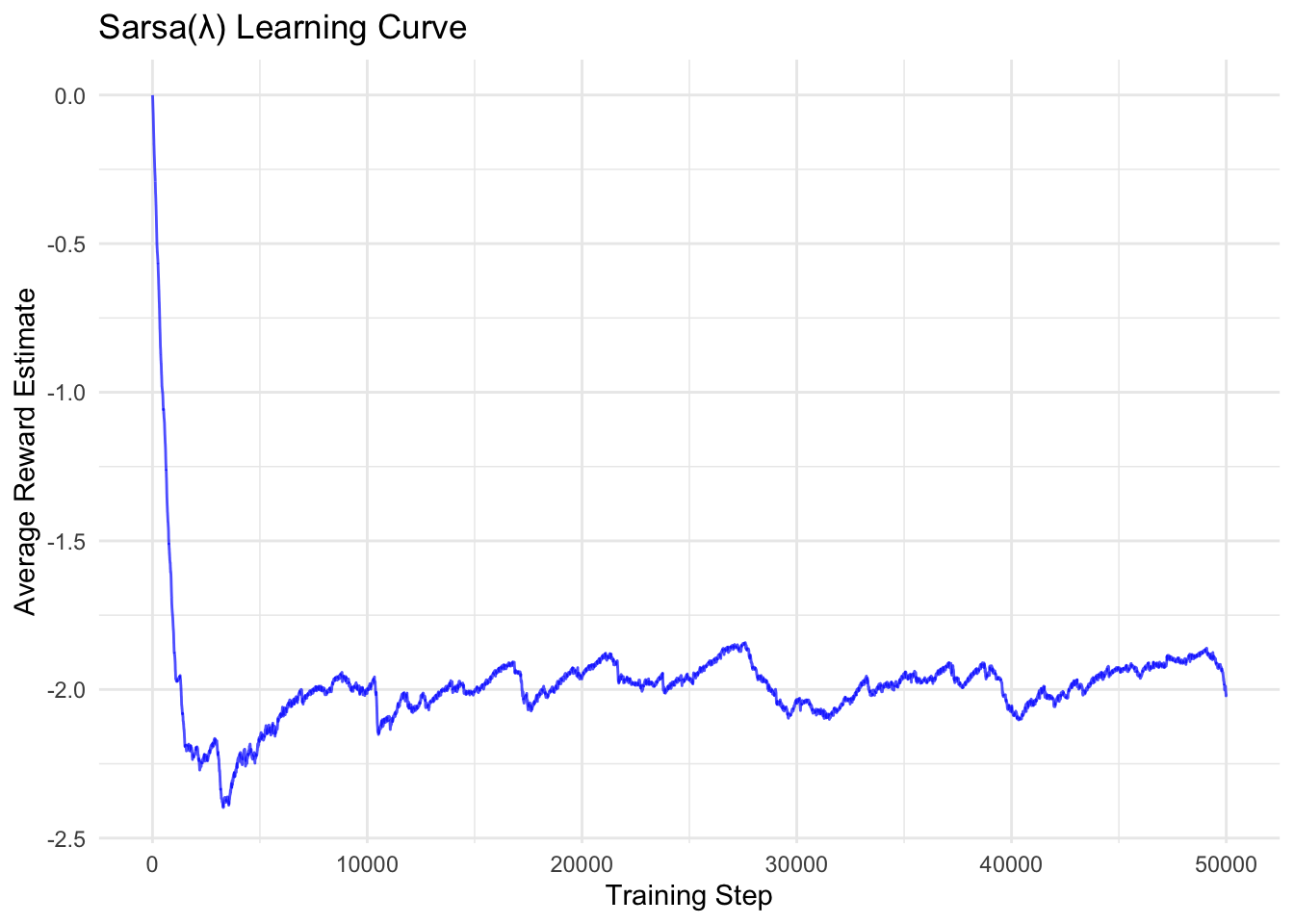
14.6 Computational and Performance Considerations

The primary advantage of using eligibility traces is improved data efficiency. By propagating information from a single experience to multiple preceding states, TD(\(\\lambda\)) and Sarsa(\(\\lambda\)) often converge significantly faster than their one-step counterparts, especially in problems with sparse rewards or long-delayed consequences. This can be critical in real-world applications where data collection is expensive or time-consuming.

However, this benefit comes at a computational cost. The one-step update only modifies a single entry in the value table. In contrast, the eligibility trace update requires iterating through and modifying every entry in the value table at each time step. For problems with very large state-action spaces, this can be prohibitively expensive. In practice, this is often mitigated by only updating traces that are above a small threshold, as very old traces contribute negligibly to the update. With the advent of deep reinforcement learning, more sophisticated methods inspired by eligibility traces are used to propagate credit through neural network weights.

Furthermore, eligibility traces introduce a new hyperparameter, \(\\lambda\). The optimal value of \(\\lambda\) is problem-dependent and often requires tuning. A high \(\\lambda\) can speed up learning but may also introduce higher variance in the updates, as they become more like Monte Carlo updates. A low \(\\lambda\) provides more stable but potentially slower learning. The choice of \(\\lambda\) reflects a bias-variance trade-off, where higher values reduce the bias of bootstrapping but increase the variance from relying on longer reward sequences.

14.7 Conclusion

Eligibility traces represent a fundamental and powerful concept in reinforcement learning, elevating simple one-step TD methods into more sophisticated algorithms capable of multi-step credit assignment. By maintaining a decaying record of past states, they enable a single TD error to update a whole chain of preceding value estimates, effectively accelerating the propagation of learned information. As demonstrated, this mechanism is not limited to the traditional discounted setting; it integrates seamlessly with the average reward formulation by using the differential TD error as its learning signal. Algorithms like Average Reward Sarsa(\(\\lambda\)) are therefore highly effective tools for solving continuing tasks where long-term performance is paramount. While they introduce additional computational complexity and a new hyperparameter, the resulting improvements in data efficiency and convergence speed make eligibility traces an indispensable component of the modern reinforcement learning toolkit.